Aim:-That company makes medicine for heart disease.We have to predict whether or not the patient has heart disease?We need to apply all five different machine learning models Logistic Regression, K-Nearest Neighbours Classifier,Support Vector machine, Decision Tree Classifier, Random Forest Classifier on the given dataset and check the accuracy about predicting whether or not the patient has heart disease.

#---------------------------------First we Import Important Labreries For our Model.---------------------------------
import pandas as pd
import numpy as np

from sklearn.linear_model import LogisticRegression
from sklearn.neighbors import KNeighborsClassifier
from sklearn import svm
from sklearn.tree import DecisionTreeClassifier
from sklearn.ensemble import RandomForestClassifier

from sklearn.metrics import accuracy_score,confusion_matrix
from sklearn.preprocessing import StandardScaler
from sklearn.model_selection import train_test_split
from matplotlib import pyplot
from sklearn.metrics import mean_squared_error;
import seaborn as sns
import matplotlib.pyplot as plt

--------------------Data Preprocessing--------------------

#----------------------------------------Importing the file into our model-----------------------------------------

db = pd.read_csv("/Users/macbook/Documents/Data Science/Indroduction To Machine learing /Project 1/heart.csv")
db.head()
db.describe()          #We use it to describe our csv file and

#------------------------------------------Data Cleaning Opreation----------------------------------------------
db.isnull().sum()                    # We cheack for null value in our data
db.info()
#db.astype(float)                     # We convert all the values into float
db.info()

#-------------------------------------------Feature And Target Values--------------------------------------
feature = list(set(db.columns)- set(["output"]))
target = list(["output"])

x = db.loc[:,feature].values            # loc is label-based, which means that you have to specify rows and columns 
y = db.loc[:,target].values             # based on their row and column labels.                                     

#---------------------------------------------Train-Test Split--------------------------------------------------------

train_x,test_x,train_y,test_y = train_test_split(x,y,test_size = 0.30,random_state = 1)

#----------------------------------------------Base Prediction --------------------------------------------------
base_pred = db[target].mean().values
base_pred = np.repeat(base_pred, len(test_y))

base_rmse = (mean_squared_error(test_y, base_pred))**0.5      # Base RMSE is used to it tells you how concentrated 
print("The Base Root Mean Squared Error Is::",base_rmse)      # the data is around the line of best fit.

#------------------------------------------Now We scale the split-----------------------------------------------------
scaler = StandardScaler()
scaler.fit(train_x)
scaler.fit(test_x)

train_x = scaler.transform(train_x)
test_x = scaler.transform(test_x)

---------------Observation Based On Graphs----------

#-----------------------------------------------------Histogram--------------------------------------------------
sns.FacetGrid(db,hue = "output",height = 5).map(sns.distplot,"age").add_legend()
plt.title("Histogram For Heart Disease Based On Age")
plt.show()

sns.FacetGrid(db,hue = "output",height = 5).map(sns.distplot,"sex").add_legend()
plt.title("Histogram For Heart Disease Based On Sex")
plt.show()

sns.FacetGrid(db,hue = "output",height = 5).map(sns.distplot,"cp").add_legend()
plt.title("Histogram For Heart Disease Based On chest pain type")
plt.show()

sns.FacetGrid(db,hue = "output",height = 5).map(sns.distplot,"trtbps").add_legend()
plt.title("Histogram For Heart Disease Based On resting blood pressure")
plt.show()

sns.FacetGrid(db,hue = "output",height = 5).map(sns.distplot,"caa").add_legend()
plt.title("Histogram For Heart Disease Based On number of major vessels (0-3) colored by flourosopy ")
plt.show()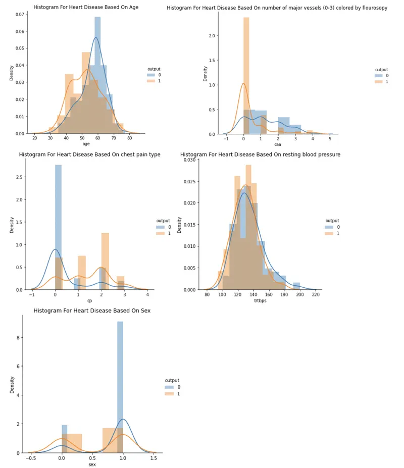

Observation Based On Histogram.

1.For the Age,the age range between 40 to 60 has maximum number of patient have a heart disease.But the age range between 60 to 80 has no heart disease.

2.For the sex type,male has maximum number of patient who have heart disease and who also dont have heart disease than female.

3.For the chest pain type,chest pain related decrease blood supply to the heart has no disease,Atypical angina has higher number of heart disease,Non-anginal pain has higest number of heart disease and Asymptomatic has lower number of heart disease.

4.For the resting blood pressure,anything above 130-140 is typically cause for heart disease.

5.For caa,number of major vessels (0-3) colored by flourosopy colored vessel means the doctor can see the blood passing through the more blood movement the better (no clots)

#------------------------------------------------Correlation Matrix-----------------------------------------------
co = db.corr()
sns.heatmap(co,annot = True,cmap="YlGnBu")

-----------------Machine learning models-----------------

1.Logistic Regression

# ---------------------------we Then implant the logestic regression on our model----------------------------------- 
lg = LogisticRegression()
lg.fit(train_x,train_y.ravel())

#-----------------------------------------Now We Predict the data--------------------------------------------- 
prediction = lg.predict(test_x)

# ------------------------Now we plot Our confusuion matrix for prediction and test data of y----------------------
confusion_matrix1 = confusion_matrix(prediction,test_y)
print(confusion_matrix1)
ax= plt.subplot()
sns.heatmap(confusion_matrix1, annot=True, fmt='g',ax=ax);
# labels, title and ticks
ax.set_xlabel('Predicted labels');ax.set_ylabel('True labels'); 
ax.set_title('Confusion Matrix'); 

# -----------------------------------Now we calculate accuracy score for our model----------------------------------

accuracy_score_LR = accuracy_score(prediction,test_y)
print("The accuracy Score are :",accuracy_score_LR)

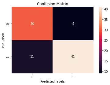
The accuracy Score are : 0.7802197802197802

The Confusion Matrix:-

2. KNeighborsClassifier

#----------------------------------------Now we classified it using K-neigbhors.------------------------------------
KNN_cla = KNeighborsClassifier(n_neighbors = 2)
KNN_cla.fit(train_x,train_y.ravel())

#-------------------------------------------Now we predict our test model---------------------------------------- 
prediction_knn = KNN_cla.predict(test_x)

#------------------------------------------- We Find Our Confusion Matrix--------------------------------------- 
confusion_matrix2 = confusion_matrix(prediction_knn,test_y)
print(confusion_matrix2)

ax= plt.subplot()
sns.heatmap(confusion_matrix2, annot=True, fmt='g',ax=ax);
# labels, title and ticks
ax.set_xlabel('Predicted labels');ax.set_ylabel('True labels'); 
ax.set_title('Confusion Matrix'); 

# ----------------------------------Now we calculate accuracy score for our model------------------------------------ 
accuracy_score_knn = accuracy_score(prediction_knn,test_y)
print("The accuracy Score are :",accuracy_score_knn)

#---------------------------------------------Plotting the effect of k--------------------------------------------
Misclassified_sample=[]
for i in range (1,20):
    knn = KNeighborsClassifier(n_neighbors=i)
    knn.fit(train_x,train_y.ravel())
    pred_i = knn.predict(test_x)
    Misclassified_sample.append((test_y != pred_i).sum())
print(Misclassified_sample)
plt.figure(figsize=(7,7))
plt.plot(range(1,20,1),Misclassified_sample,color="red",linestyle="dashed",marker="o",markerfacecolor="blue",markersize = 10)
plt.show()

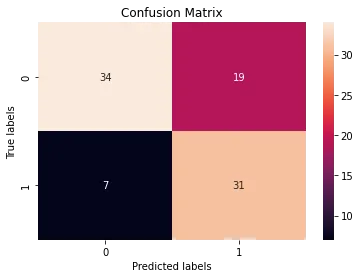
The accuracy Score are : 0.7142857142857143

The Confusion Matrix:

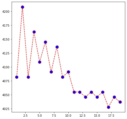
From above graph that shows the effect of value of k on the misclassified sample.As we keep increasing the value of k the misclassified values keep decresing.

3.Support Vector machine

#----------------------------------------Now we classified it using SVM.------------------------------------
svm_model = svm.SVC()
svm_model.fit(train_x,train_y.ravel())

#-------------------------------------------Now we predict our test model---------------------------------------- 

prediction_svm = svm_model.predict(test_x)

#------------------------------------------- We Find Our Confusion Matrix--------------------------------------- 

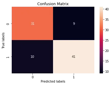
confusion_matrix3 = confusion_matrix(prediction_svm,test_y)
print("The Confusion Matrix:n",confusion_matrix3)

ax= plt.subplot()
sns.heatmap(confusion_matrix3, annot=True, fmt='g',ax=ax);
# labels, title and ticks
ax.set_xlabel('Predicted labels');ax.set_ylabel('True labels'); 
ax.set_title('Confusion Matrix'); 

# ----------------------------------Now we calculate accuracy score for our model------------------------------------ 
accuracy_score_svm = accuracy_score(prediction_svm,test_y)
print("The accuracy Score are :",accuracy_score_svm)

The accuracy Score are : 0.7912087912087912

The Confusion Matrix:

4.Decision Tree Classifier

#----------------------------------------Now we classified it using Decision Treee.-----------------------------------
decision_tree = DecisionTreeClassifier(random_state=0, max_depth=4)
decision_tree.fit(train_x,train_y.ravel())

#-------------------------------------------Now we predict our test model---------------------------------------- 

prediction_DT = decision_tree.predict(test_x)

#------------------------------------------- We Find Our Confusion Matrix--------------------------------------- 

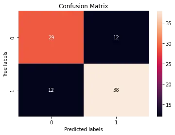
confusion_matrix4 = confusion_matrix(prediction_DT,test_y)
print("The Confusion Matrix:n",confusion_matrix4)

ax= plt.subplot()
sns.heatmap(confusion_matrix4, annot=True, fmt='g',ax=ax);
# labels, title and ticks
ax.set_xlabel('Predicted labels');ax.set_ylabel('True labels'); 
ax.set_title('Confusion Matrix');

# ----------------------------------Now we calculate accuracy score for our model------------------------------------ 
accuracy_score_DT = accuracy_score(prediction_DT,test_y)
print("The accuracy Score are :",accuracy_score_DT)

The accuracy Score are : 0.7362637362637363

The Confusion Matrix:

5.Random Forest Classifier

#----------------------------------------------Now we deploy Random Forest -----------------------------
rf = RandomForestClassifier(n_estimators=100,random_state=1)

rf.fit(train_x,train_y.ravel())

#-------------------------------------------Now we predict our test model---------------------------------------- 

prediction_rf = rf.predict(test_x)

#------------------------------------------- We Find Our Confusion Matrix--------------------------------------- 

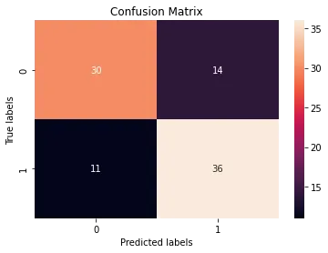
confusion_matrix5 = confusion_matrix(prediction_rf,test_y)
print("The Confusion Matrix:n",confusion_matrix5)

ax= plt.subplot()
sns.heatmap(confusion_matrix5, annot=True, fmt='g',ax=ax);
# labels, title and ticks
ax.set_xlabel('Predicted labels');ax.set_ylabel('True labels'); 
ax.set_title('Confusion Matrix');

# ----------------------------------Now we calculate accuracy score for our model------------------------------------ 
accuracy_score_rf = accuracy_score(prediction_rf,test_y)
print("The accuracy Score are :",accuracy_score_rf)

The accuracy Score are : 0.7252747252747253

The Confusion Matrix:

Now We Compare the accuracy Score for each model.

model = ["Logistic Regression", "K-Nearest Neighbours Classifier", "Support Vector machine", "Decision Tree Classifier", "Random Forest Classifier"]
accuracy = [accuracy_score_LR,accuracy_score_knn,accuracy_score_svm,accuracy_score_DT,accuracy_score_rf]
c = ['green', 'Aqua', 'Orange', 'blue', 'maroon']

fig = plt.figure(figsize = (20, 10))
plt.bar(model,accuracy,color = c,width = 0.4)

plt.title("Accuracy of All Model")
plt.ylabel("Accuracy")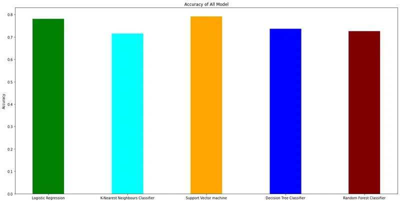

Conclusion:-

From above bar graph we can see accuracy for each model.

1.For Logistic Regression,this model is give around 78.02% accuracy. Which is slightly greater than svm model.

2.For K-Nearest Neighbours Classifier,this model is gives around 71.42% accuracy.Which is smaller than Logistic Model

3.For Support Vector Machine,this model is gives around 79.12% accuracy. The accuracy of This model is higher than all models.

4.For Decision Tree Classifier,this model is gives around 74.72% accuracy.Which is slightly higher than KNN model.

5.For Random Forest Classifier,this model is gives around 78.02% accuracy.Which is similar to logestic regression Model.

Based On Observation we can conclude that,Support Vector Mechine is best suitable for our data.Beacause it has maximum accuracy.

-----------------------------------------------------------