Development of a forward energy-based fuel consumption model of a conventional vehicle.
Development of a forward energy-based fuel consumption model of a conventional vehicle.
Objective:-
To build a simulink model and the matlab script to achive the below objectives:
a)To tabulate the fuel economy numbers (kmpl) for UDDS and HWFET cycle. This forms the baseline numbers for comparing with the future hybrid version.
b)To Plot the time trace for engine, transmission input, transmission output and wheel speed on one plot.
c)To Plot engine torque, engine power, fuel rate and fuel consumption using subplots.
d)To Plot accelerator and brake pedal, gear command, vehicle desired and actual speed, vehicle distance using subplots.
e)To Plot the engine operating points on the engine fuel map.
f)Write down appropriate brief comments on each of these plots, describing the vehicle behavior throughout the drive cycle.
g)To Generate the plots for both drive cycle
Project Description:-
Major Components and parts of the conventional vehicle:-
An automobile has several numbers of parts. But there are four essential components of automobile. These are:
1. The Chassis.
2. The Engine.
3. The Transmission System.
4. The Body.
Apart from these four essential parts of automobile, there are controls and auxiliaries.
The controls are meant for controlling the movement of the vehicle. The auxiliaries are additional components meant for providing comfort to the user of the automobile.
1. The Chassis.
The chassis of an automobile incorporates all the major assemblies consisting of an engine, components of transmission system such as clutch, gearbox, propeller shaft, axles, a control system such as brakes and steering, and suspension system of the vehicle.
In other words, it is the vehicle without its body.
2. The Engine.
The engine is the source of motive power to an automobile. Obviously, it is a very important part of the automobile because in the absence of an engine, the automobile may not move at all, and its basic function of transporting passengers or goods would be defeated.
The power of the engine determines the working of the automobile. In the same manner, the efficiency of the engine determines the efficiency of an automobile.
The engine, nowadays, is invariably an internal combustion engine. This may be a spark-ignition engine consuming petrol as fuel.
Alternatively, it could be a compression ignition engine using diesel as fuel.
3. The Transmission System.
The transmission system transmits power developed by the engine to the road wheels. The power available as output from the engine is in the form of rotation of the crankshaft.
This movement is to be transferred to the road wheels to cause their rotary motion. Their rotary motion makes possible the movement of the vehicle.
The transmission system consists of different parts. These include clutch, gearbox, propeller shaft, differential and axle, live axle to be more precise.
The road wheels are at the ends of the axle. The motion is transmitted through these parts. Every part of the transmission system performs its own function.
i. Clutch.
The clutch, part of the transmission system is next to the crankshaft. It is a mechanism enabling the rotary motion of one shaft transmitted to the second shaft ‘at will.’
When the engine starts, it should not be connected to road wheels, i.e., these should not start moving as soon as the engine starts.
Secondly, this motion should be smoothly transferred so that passengers in the car do not feel discomfort, and its mechanism is not spoiled.
ii. Gearbox.
The gearbox is the component of the transmission system next to the clutch. It has got a gear train, and it provides different gear ratios. These ratios determine the rotary speed of output shaft from the gearbox.
The torque transmitted to the road wheels gives rise to a propulsive force or (tractive effort) between these and the road. When starting from rest, a large tractive effort is required.
This makes essential the introduction of considerable ‘leverage’ between the engine and the wheels so that torque from the engine, which is almost constant, produces the large tractive effort.
This ‘leverage’ is provided by the gearbox.
Different gear ratios available in the gearbox can provide the required tractive effort to overcome the resistance faced by the automobile under different conditions.
Propeller shaft transmits the output from the gearbox to the axle. This axle may be in the rear or in the front or in some cases both the rear and front axle may receive output from the gearbox.
The output from the gearbox is in the form of rotary motion of the shaft, and this motion is transferred to the axle.
iii. Differential.
The differential is the next component of the transmission system. The motion of propeller shaft is fed to the differential which turns it through 90 degrees. This is essential as the axle is at 90 degrees to the propeller shaft.
The function is performed with the help of a pinion and a gear. Another important function of the differential is to reduce the speed of inner wheels and at the same time, enhance the speed of outer wheels by the same amount.
This is required when the automobile is moving on a curved path. On a curved path, the outer wheels are required to traverse a circle of a bigger radius than the inner wheels.
This means that the outer wheels are required to traverse larger distance as compared to inner wheels. As the automobile is to move as a single unit, all the four wheels must travel together.
Therefore, the outer wheels should travel larger distance and inner wheels should travel smaller distance in the same time period.
Hence, the variation in the speed of inner and outer wheels is needed. This is performed by the differential with the help of sun and planet gear system.
iv. Axle.
The axle is the next component of the transmission system. The axle receiving power from the engine is termed as ‘live’ axle. It is in two halves.
The ends of the axle have road wheels connected to it. These road wheels are in direct contact with the road surface. The body of the automobile is above the axle.
The axle also takes up the various loads including the weight of the automobile. It also transmits motion to the road wheels.
FORWARD MODEL FOR A CONVENTIONAL VEHICLE:-
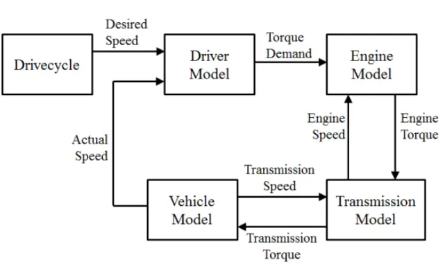
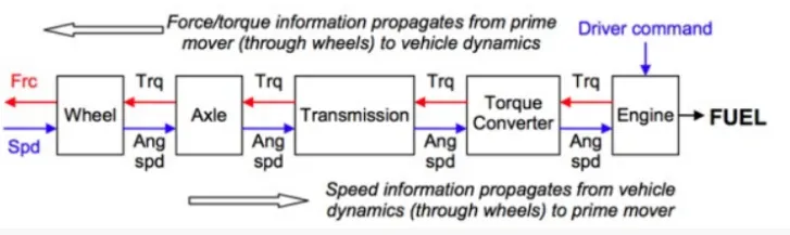
The vehicle model used in this investigation features a conventional powertrain that is found on majority of the vehicles on the road. It contains an ICE, clutch, manual transmission, and final drive. It also includes environment losses such as aerodynamic drag and rolling resistance. For the purpose comparing the two types of modelling approaches however, only the ICE displacement and final drive ratio is made scalable, and used as decision variables by the optimiser to minimise the cost function.
The forward-facing (dynamic) vehicle model is shown in above figure.It is observed that the transfer of power information is bi-directional in the forward-facing model, i.e. the direction of effort (torque) is opposite to the direction of flow (speed).
A forward-facing vehicle model features a driver model that provides torque demand in the form of desired ICE torque and brake torque, to meet the speed trace from a drivecycle. The topology of the forward-facing model that is used in this investigation is shown in above model.
A basic driver model typically uses one or more Proportional-Integral (PI) controllers to achieve the torque demand, with reference to the desired speed trace. This is discussed further in the next section. The torque produced by the ICE propagates through the transmission and final drive ratios, before ending up as torque applied at the wheels. This is then exerted to the vehicle mass via force on the tyre contact patch. The vehicle speed that results from the applied force is propagated back through the drivetrain, and returns to the ICE as angular velocity at the crankshaft. Brake torque is applied directly at the wheels.
Forward-facing models provide insight into the vehicle model drivability, and it captures the limits of the physical system. It also makes control development and implementation on HIL systems easier However, with the presence of multiple state equations in a typical forward-facing model, the vehicle speed (and subsequently drivetrain angular velocity) is computed via multiple state integration, resulting in the need
to run the simulation in smaller time steps.
Once both engine torque (or the Brake Mean Effective Pressure, BMEP) and speed have been determined, a 0D black box model of the engine can be used to find the instantaneous fuel consumption or emission rate, as shown . Finally, instantaneous fuel consumption and emission rate are integrated over the driving cycle to obtain cumulative data.Obviously, this approach neglects all the dynamic phenomena considering transient conditions as a sequence of stationary states; therefore it is often used only for a first preliminary estimation of the fuel consumption or engine emissions of a motor vehicle, although the simulation results can differ significantly from the experimental data due to these simplifying assumptions.
*******************************************************************************************************
VEHICLE MODELLING USING MATLAB:-
Initial Modelling:-
%%%%%%%%%%%%%%%%%%%%%%%%%%%%%%%%%%%%%%%%%%%%%%%%%%%%%%%%%%%%%%%%%%%%%
%% Skill-Lync -> Hybrid Drives Development
% Project 1 - Conventional Vehicle Model
% By - Ullekh Gambhira

% Description:

%% Initialization File
% Initialization file for loading the variables for the Conventional vehicle simulation model

%% Vehicle Parameters
M = 1500;       % Vehicle weight [kg]
Cr = 0.015;     % Rolling resistance coefficient
Rw = 0.35;      % Rolling radius [m]
Cd = 0.33;      % Drag coefficient
Af = 2;         % Frontal area [m2]
rhoa = 1.225;   % Air density [kg/m3]
Vwind = 0;      % Wind velocity [kmph]
g = 9.81;       % Gravitational acceleration [m/s2]
theta = 0;      % Slope [deg]
myu_road_tire = 1; % Coefficient of friction between tire - road interface

%% Powertrain Parameters
FDR = 3.73;                         % Final Drive Ratio / Diff Ratio
DiffEff = 0.99;                     % Differential efficiency (assumed independent of operating conditions)

NumGear = 4;                        % Number of gears in transmission
TransGear = [1:NumGear];            % Transmission Gears
TransRatio = [3.06, 1.62, 1, 0.7];  % Corresponding Transmission ratios
TransEff = 0.90;                    % Transmission efficiency (assumed independent of operating conditions)

TC_SR = [0, .5, .6, .7, .8, .87, .92, .94, .96, .97, 1];   % Torque Converter Speed Ratio (Matlab default) -> TurbSpd/PumpSpd
TC_TR = [2.232, 1.5462, 1.4058, 1.2746, 1.1528, 1.0732, 1.0192, 1, 1, 1, 1];   % Torque Converter Torque Ratio (Matlab default) -> TurbTrq/PumpTrq
TC_Cf = 1e-4 * [.72558, .66322, .63463, .59042, .51331, .4144, .29287, .22444, .12186, .04386, 0]; % Torque Converter Capacity Factor (Matlab default) -> PumpTrq/PumpSpd^2 [Nm/rpm^2]

load Vehicle_Data/Engine_data_1_9L_Saturn_95kW
load Vehicle_Data/Trans_Shift_map

%% Driver Parameters
Kp = 10;                    % P gain for driver PI model
Ki = 1;                     % I gain for driver PI model
Drive_Cycle_Select = 1;     % Drive cycle selection

% Drive cycle values in m/s

if Drive_Cycle_Select == 1
    load DriveCycles/UDDS;

elseif Drive_Cycle_Select == 2
    load DriveCycles/HWFET;

elseif Drive_Cycle_Select == 3
    load DriveCycles/FTP;

elseif Drive_Cycle_Select == 4
    load DriveCycles/US06;

elseif Drive_Cycle_Select == 5
    load DriveCycles/NEDC;

elseif Drive_Cycle_Select == 6
    load DriveCycles/WLTP;

end

time_end = cyc_time(end);
vel_end = cyc_vel(end);
In this above matlab script, all the input parameters which are mainly required for a conventional vehicle are discussed. As we can see, Vehicle parameters, Powertrain parameters, Driver parameters including the Drive cycles are also scripted. We can choose different drive cycles by changing the varialbe "Drive_Cycle_Select = 1; % Drive cycle selection"
| Drive cycle Variable | Drive Cycle selected |
| 1 | UDDS |
| 2 | HWFET |
| 3 | FTP |
| 4 | US06 |
| 5 | NEDC |
| 6 | WLTP |
So according to our driving conditions we can choose our own drive cycle easily. Here in this project the all the important vehicle parameters are detailedly explained for UDDS and HWFET drive cycles.
SIMULINK MODEL:-
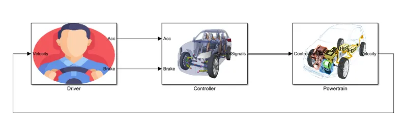
These are the three important subsystems or blocks, which are used to model the conventionall vehicle. The three important blocks are Driver block, Controller block and the powertrain block. We will discuss the blocks one by one below:-
1) Driver Block:-
When the driver block is opened, we will get the following sub blocks as follows:-
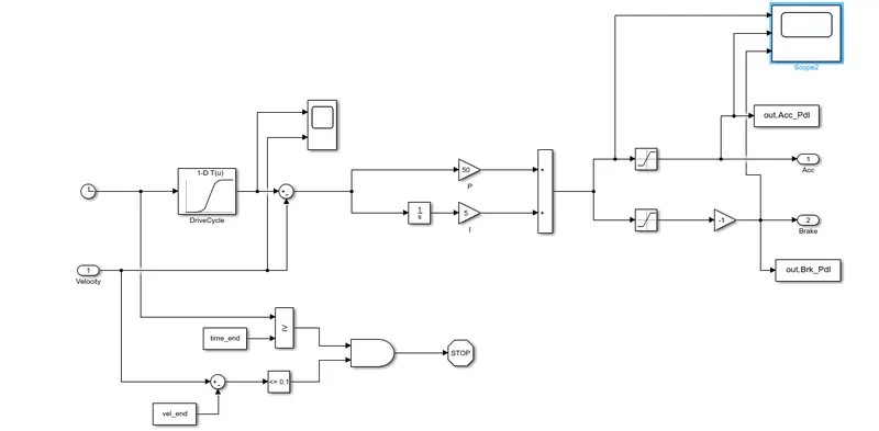
A driver model is a mathematical model which replicates the. functionality of a driver( controlling , monitoring and stabilizing a vehicle )during various maneuvers.It is modeled using a ‘Driver’ block, which is a basic PI controller that generates accelerator and brake pedal outputs to match the desired and actual vehicle speeds. In this we use drive cycles fro the based on these results of fuel consumption and emissions the vehicle gets certified and it also forms a basis of uniform asessment. It is based on time, velocity then its all integrate and creates output accelration pedal and brake pedal.
2) Controller block:-
When the controller block is opened, we will get the following sub blocks as follows:-
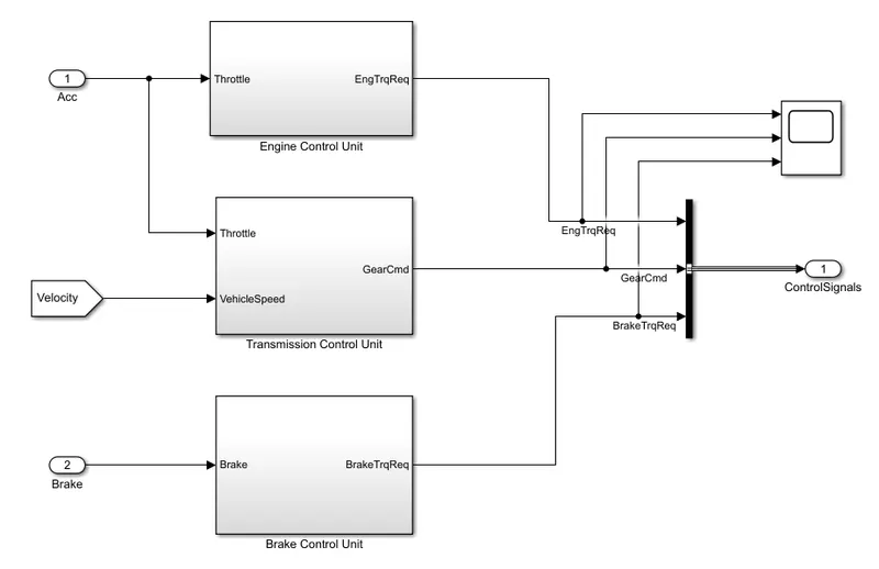
The engine control, Transmission control and the Brake control are the main units required for a conventional vehicle. Now we can see the indiviual blocks and their models below:-
a)Engine control unit:-
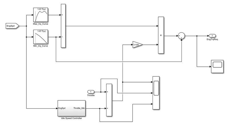
For the engine control unit, the accleration is given as the input. In this engine control unit all the necessary parameters which are required for the running performance of the engine is modelled. And hence for the given engine speed the Engine torque and idle speed can also be found out with the help of this engine control block.And hence the required throttle can be found out with in the model. And with the help of the scope block, all the all the parameters like Engine torque, idle speed and the throttle performances can be analysed graphically.
b) Transmission Control unit:-
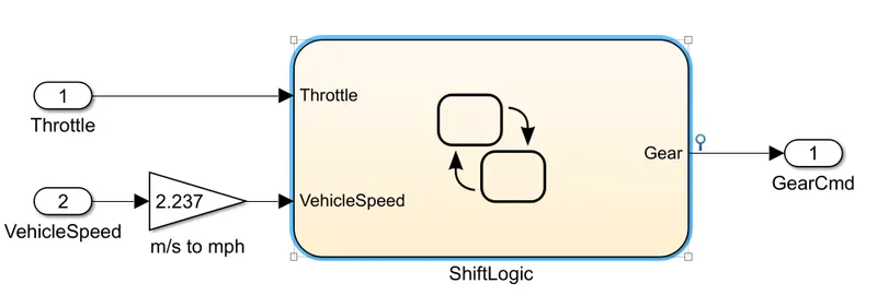
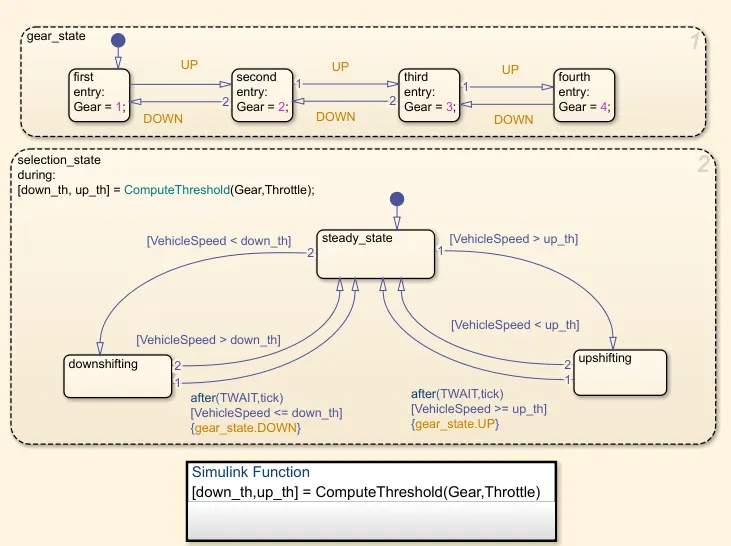
Hear the gear shifting Logics are done with the help of matlab scripting. The vehicle speed is given as the input for the gear shifting logic and depending upon the speed variation the respective gear is selected and is chosen to run the vehicle .As we can see in the second image the gear shifting logic is provided and the different speeds are analysed and depending upon the speed the correct gear is selected.It will automatically shift to the lower gears when the speed reduces to the optimum value which is defined in the shift logic.The out put signal from this block is also used to modify the powertrain parameters.
c)Brake control unit:-
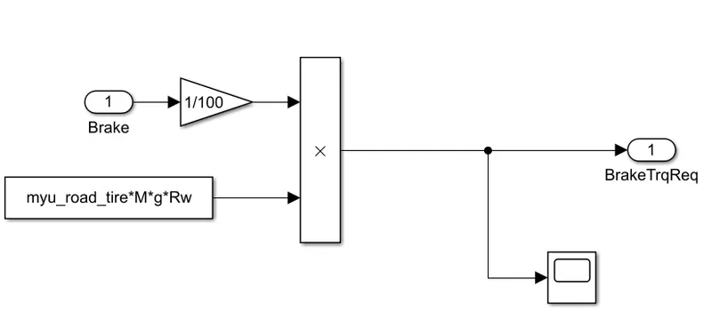
In this block, the brake torque is calculated and all the three outputs from the engine, transmission and the brake control units are then fed into the powertrain block:-
3) Powertrain Block:-
The main components which are used in the power train blocks are:-
a)Engine Block
b)Transmission Block
C)Differential Block
d)Wheels Block
e) Vehicle dynamics Block
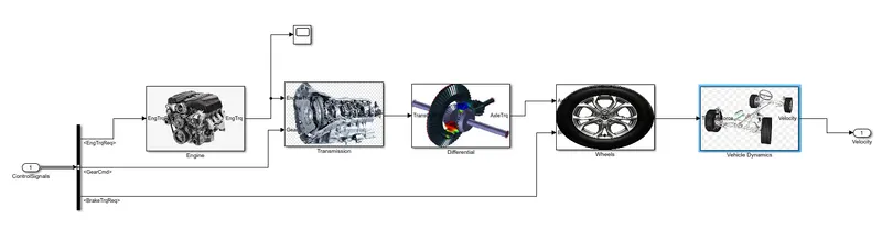
a)Engine Block:-
When you open the engine block, the following sub blocks will be modelled there:-
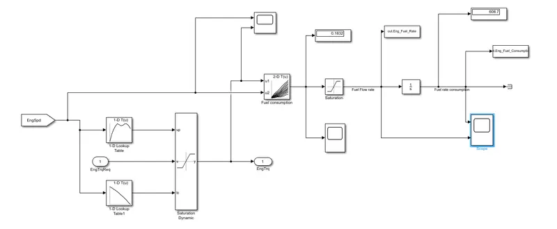
The engine speed is given as the input for the engine block and for that engine speed given, the fuel consumption and the fuel flow rate can be calculated in this engine block. The maximum torque and the minimum torque are taken up into a 1D lookup table and they are fed into the saturation dynamic block so that both that the optimum values are chosen by the saturation dynamic block and we will obtain the final engine torque value.
And then the final engine torque and engine speed is fed into the fuel consumption 2D lookup table for those consumption again a saturation block is chosen to to obtain the minimum and maximum limits and the output of the saturation lord will give you the fuel flow rate when that fuel flow rate this integrated with the help of the integrator block actual fuel rate consumption can be found out and then the signal is terminated.
Two 'To workspace' blocks are used to get the engine fuel rate and the engine fuel consumption to the matlab workspace with the help of two workspace block. This is the working of the engine block Model.
b)Transmission Block:-
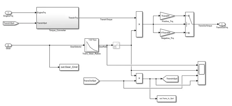
The transmission model comprises from the given gear input and for the given gear inputs, the gear ratios are calculated and finally the transmission output speed and the transmission out put torque are calculated. The transmission output signal is taken as the next input for the vehicle dynamics block.
The another important sub block used is the 'Torque converter block'. When you open the torque converter block, the following blocks will get displayed.
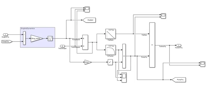
A torque converter is a type of fluid coupling that transfers rotating power from a prime mover, like an internal combustion engine, to a rotating driven load. In a vehicle with an automatic transmission, the torque converter connects the power source to the load. It is usually located between the engine's flexplate and the transmission. The equivalent location in a manual transmission would be the mechanical clutch.
The main characteristic of a torque converter is its ability to increase torque when the output rotational speed is so low that it allows the fluid coming off the curved vanes of the turbine to be deflected off the stator while it is locked against its one-way clutch, thus providing the equivalent of a reduction gear. This is a feature beyond that of the simple fluid coupling, which can match rotational speed but does not multiply torque and thus reduces power.
c)Differential Block:-
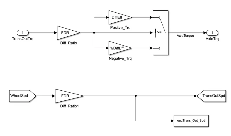
In this differential block, for the given transmission output torque, the axle torque is calculated. A switch block is connected in between the positive and negative torque gain blocks, so that only the positive torque is taken into the consideration and for that positive torque , the axle torque is calculated.
d) Wheel Block:-
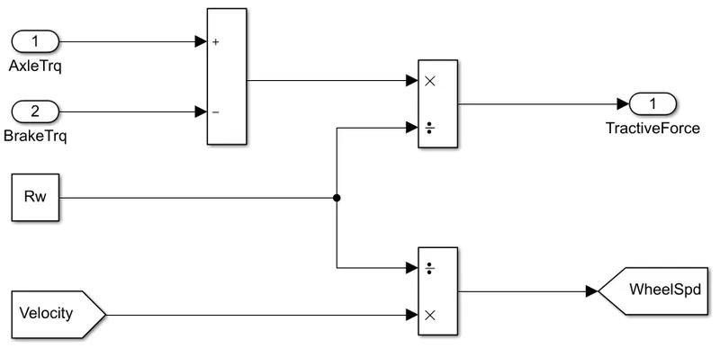
Here in this wheel block, For the provided Axle and brake torques, the tractive force and for the obtained velocity, the wheel speed is also calculated.The brake torque from the control model is subtracted from the Axle torque and divides from the rolling radius to determine the Tractive force. And hence we can obtain the Tractive force and the wheel speed from this above model.
e)Vehicle Dynamics Block:-
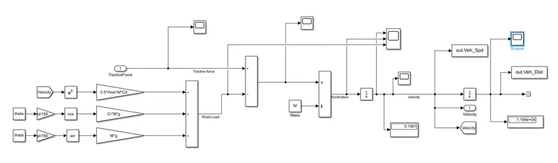
The vehicle movement is described by the longitudinal forces equation:
where:
Ft [N] – traction force
Fi [N] – inertial force
Fs [N] – road slope force
Fr [N] – road load force
Fa [N] – aerodynamic drag force
The traction force can be regarded a a “positive” force, trying to move the vehicle forward. All the other forces, are resistant, “negative” forces which are opposing motion, trying to slow down the vehicle.
Here,
The inertial (resistant) force [N] is given by the equation:
The road slope (resistant) force [N] is given by the equation:
The road load (resistant) force [N] is given by the equation:
The aerodynamic drag (resistant) force [N] is given by the equation:
Replacing (4) in (1) and rearranging the terms, gives:
By integrating equation (10) we obtain the vehicle speed [m/s]:
a) The UDDS drive signal from the 'Driver block' :-
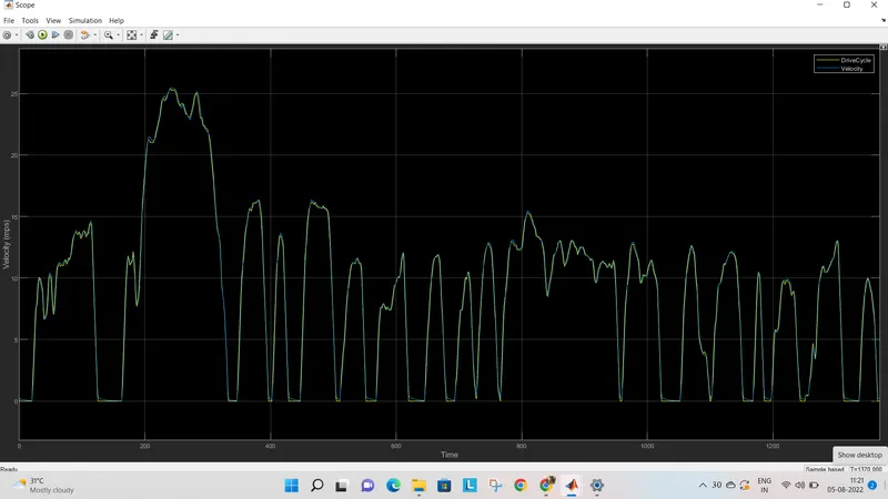
From the driver block we will get the curve for the UDDS drive cycle which we have implemented in the matlab script as we can clearly see that the velocity is higher in between the values of time 200 to 300 seconds so we will discuss with this maximum velocity for our upcoming graphs and we can verify whether our script and model is behaves depending upon the speed variations provided in our UDDS drive cycle. We can also see that the velociity curve and the drive cycle curve matches toogether.
b) Graph of Accleration Pedal and Brake pedal from Driver block model:-
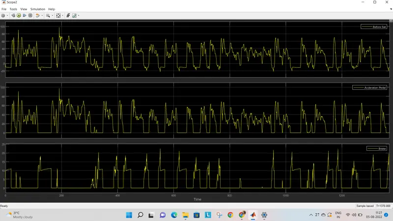
In this graph the plots for the acceleration pedal and the brake pedal are plotted. When we compared these plots to the previous plot that is with our UDDS drive cycle. that acceleration is higher in between the time range of 200 to 300 seconds again when we look into the graph of acceleration pedal and brake pedal we can experience the same heights in the acceleration padel between the period of 200 to 300th seconds and when the vehicle is accelerated between these time period we can see the brake pedal the value remains ZERO.And hence its very clear that the brake pedal values are zero, whenever there is a accleration. (ie., our vehicle is in running mode)
c) Engine Torque graph from Controller block->Engine control unit:-
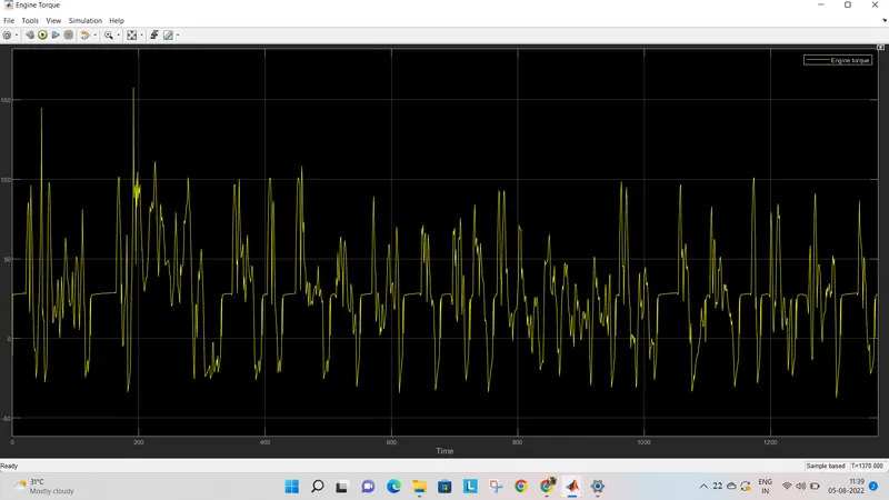
The above graph is obtained from the engine control unit block and its showing us the graph for the Engine torque values. We can see that intially the engine torque values are high sice at the start of the vehicle. And similarly you can compare this with the brake pedal graph after the brake pedal graph we can experience a little higher torque values, since the vehicle will start from 1st gear.
d) Brake graph from the Brake control unit:-
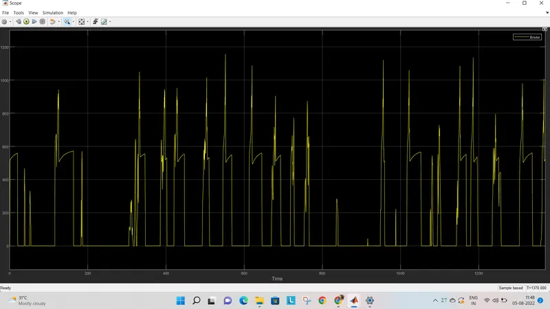
This graph provides us the value of brake, as we can see that the brake value is zero whenever we have the higher amount of acceleration given to the vehicle. As when we compared this graph with our first graph which is our you UDDS drive cycle ,whenever we experience the higher acceleration that is in between the time seconds of 200 to 300, we will experience zero brake value for the same time frame 200 to 300 seconds (ie., No brake is applied between the accleration period)
e) The Engine torque, Gear command & Brake graphs:-
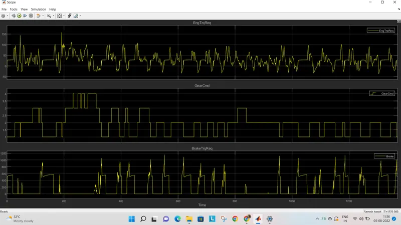
This graphs compares the Engine torque, Gear command and the Brake torque. As we can see, during the time period of 200 to 300 seconds, the vehicle is running at the higher speeds and hence we can see that the gear value is 4 in the gear command graph. Similarly when the vehicle is running at higher gear, we can see the brake values as zero, as no brake is applied.
f) Fuel consumption and Fuel flow rate values from the Engine block:-
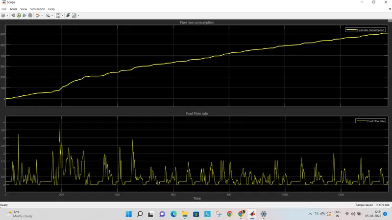
This graph represents the fuel consumption and the fuel flow rate of the vehicle. As we can see in the first plot the fuel is consumed over the period of time as the vehicle moves continously over the period of time. And similarly we can experience the fuel flow rate in the second graph, as the fuel flow rate rises in between the 200th second we can see a similar rise in the fuel rate consumption graph.And it is clear that, the fuel consumption will get increase over the period of time as the car is in acclerated stage.
g) Velocity, Acclertion and Roadload graphs from the vehicle dynamics block:-
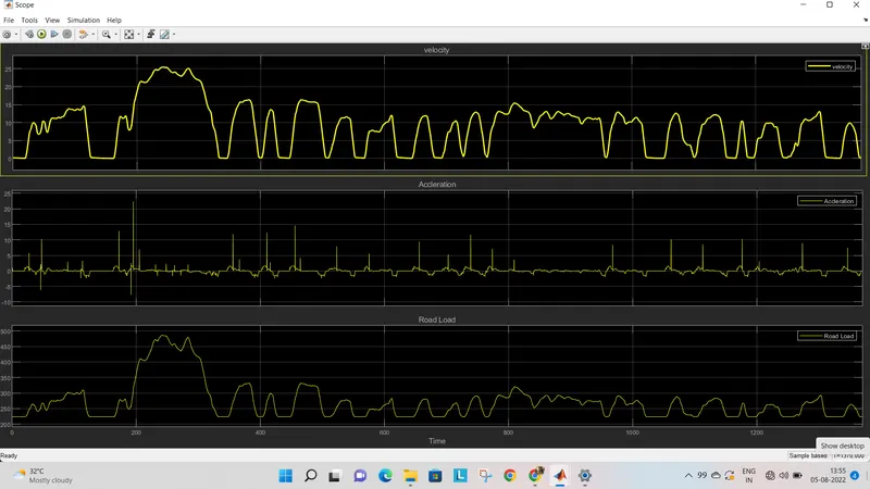
This graph represents the velocity,acceleration and Road load for the conventional vehicle we have taken. The first plot represents the velocity, the second plot represent the acceleration, and the third plot represent the road load .As we can clearly see, when the velocity is higher due to the accleration of the vehicle, the Aerodynamic forces variables will also rise and hence the road load will be higher and hence it is clearly seen in between the type range of 200 to 300th second.
h) Distance covered by the vehicle:-
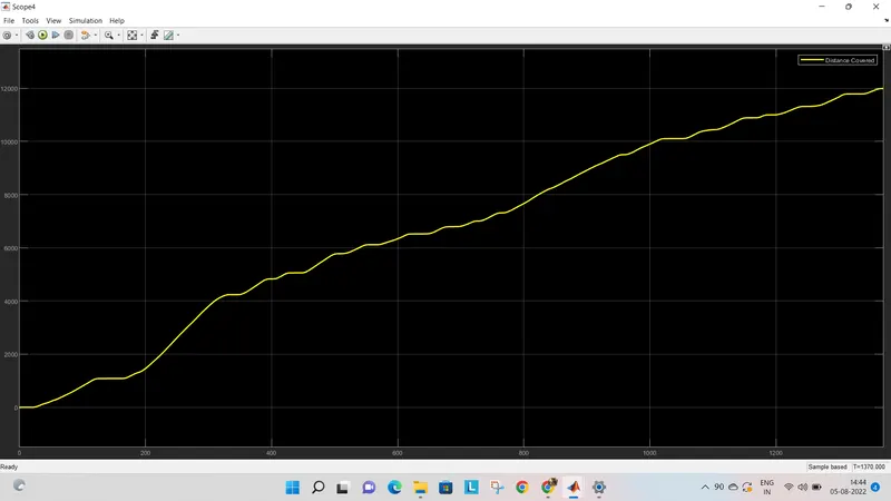
From the graph we can see that the distance travelled by the vehicle for about 1369 seconds.
OUTPUTS FOR HWFET DRIVE CYCLE:-
Similarly, all the graphs are obtained for the HWFET drive cycle:-
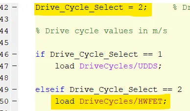
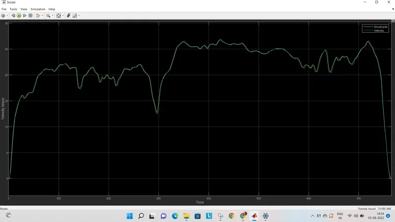
a) The HWFET drive signal from the 'Driver block' :-
b) Graph of Accleration Pedal and Brake pedal from Driver block model:-
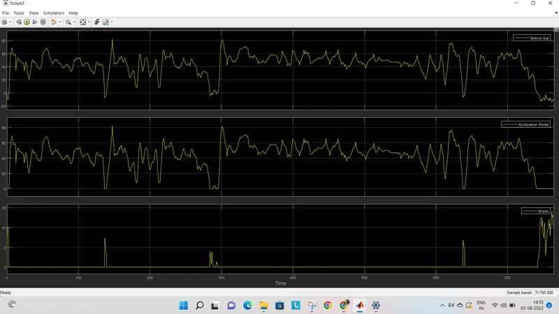
Here as you can see, as most of the time, the vehicle will be in accleration, so the brake pedal values are almost zero for longer times.
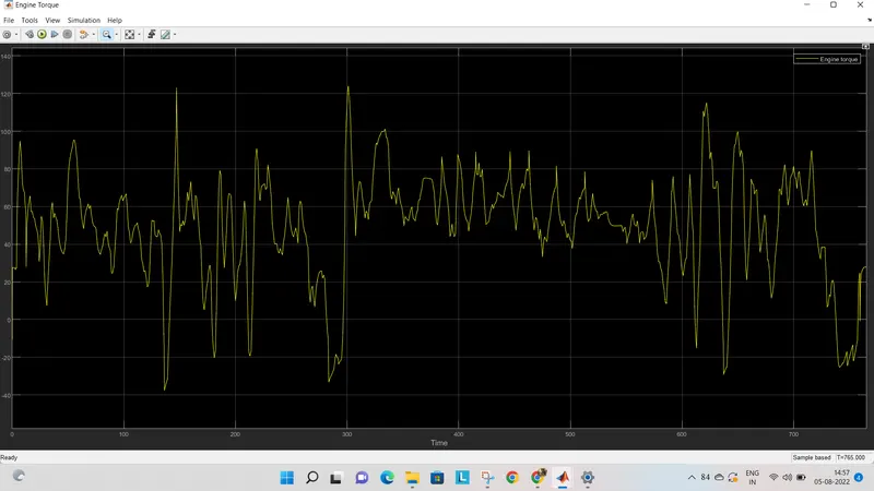
c) Engine Torque graph from Controller block->Engine control unit:-
d) Brake graph from the Brake control unit:-
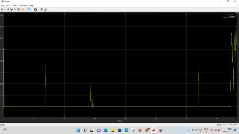
Since it is a highway drive, Brake values are almost zero for every cycles.
e) The Engine torque, Gear command & Brake graphs:-
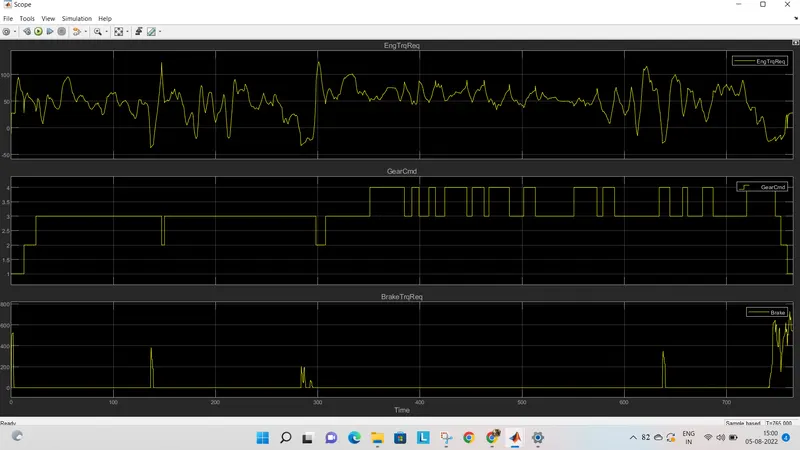
As seen in the graph, the vehicle mostly drives with the gigher gear value ie., 4. And the brake is applied for only few times.
f) Fuel consumption and Fuel flow rate values from the Engine block:-
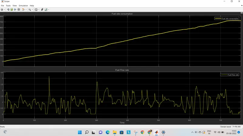
As we can see, the fuel consumption is getting higher by higher when the vehicle covers distance.
g) Velocity, Acclertion and Roadload graphs from the vehicle dynamics block:-
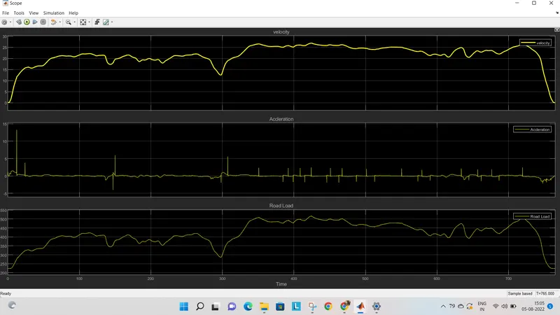
As we can see that, the velocity matches our given HWFET drive cycle and due to the higher aerodynamic force in the highway drive, we will experience a higher road load and is shown in the graph.
Post Processing Matlab Script:-
%%%%%%%%%%%%%%%%%%%%%%%%%%%%%%%%%%%%%%%%%%%%%%%%%%%%%%%%%%%%%%%%%%%%%
%% Skill-Lync -> Hybrid Drives Development
% Project 1 - Conventional Vehicle Model
% By - Ullekh Gambhira

% Description:
% The following file is to used with the Initialization file and Simulink
% results for post-processing of the data.
% The file is incomplete, has some examples of how the data is imported
% into a readable format, data analysis and plotting examples.
% Based on the project task, use commands in a similar format as given
% below, to analyse the data and generate required plots.
% You can change variable names if desired

%% Post-Processing File
%  File for post-processing the Conventional vehicle simulation model data

%% Renaming variables
Time = out.tout;
Acc_Pdl = out.Acc_Pdl;          % Accelerator pedal [%]
Brk_Pdl = out.Brk_Pdl;          % Brake pedal [%]
Gear_Cmd = out.Gear_Cmd;        % Transmission gear
Trans_In_Spd = out.Trans_In_Spd*30/pi;  % Transmission input speed [rpm]
Trans_Out_Spd = out.Trans_Out_Spd*30/pi;% Transmission output speed [rpm]
Eng_Trq = out.Eng_Trq;          % Engine brake torque [Nm]
Eng_Spd = out.Eng_Spd*30/pi;    % Engine speed [rpm]
Eng_Fuel_Consump = out.Eng_Fuel_Consumption;    % Engine fuel consumption [g]
Veh_Dist = out.Veh_Dist/1000;   % Distance traveled by vehicle [km]
Veh_Spd = out.Veh_Spd*18/5;     % Vehicle speed [kmph]


%% Data Analysis
Eng_Pwr = Eng_Spd*pi/30*Eng_Trq/1000;   % Engine brake power [kW]
rho_petrol = 0.7197;                    % Density of petrol [kg/L]
kmpl = Veh_Dist(end)/(Eng_Fuel_Consump(end)/1000/rho_petrol);    % Fuel economy [kmpl]


%% Plotting vehicle characteristics time trace
figure()
subplot(3,1,1)
hold on
grid on
plot(Time, Acc_Pdl, 'linewidth', 1, 'Color', 'black');
plot(Time, Brk_Pdl, 'linewidth', 1, 'Color', 'red');
ylabel('Pedal [%]')
xlim([0, Time(end)]);
legend('Accel','Brake');
subplot(3,1,2)
hold on
grid on
plot(Time, Trans_In_Spd, 'linewidth', 1, 'Color', 'black');
plot(Time, Trans_Out_Spd, 'linewidth', 1, 'Color', 'red');
ylabel('Speed [rpm]')
xlim([0, Time(end)]);
ylim([0, 6000]);
legend('Trans Input','Trans Output');
subplot(3,1,3)
hold on
grid on
plot(Time, Gear_Cmd, 'linewidth', 1, 'Color', 'black');
xlim([0, Time(end)]);
xlabel('Time [s]');
ylabel('Gear');

%% Plotting engine operating points on engine fuel map
figure('Name','Engine Operating Points');
hold on
grid on
title('Engine Operating Points','fontsize',12);
p1=plot(Eng_map_spd*30/pi,Eng_max_trq,'linewidth',2,'color','r');
p2=line([Eng_map_spd(end)*30/pi Eng_map_spd(end)*30/pi],[0 Eng_max_trq(end)]);
set(p2,'linewidth',1,'linestyle','--','color','k');
p3=line([Eng_map_spd(1)*30/pi Eng_map_spd(1)*30/pi],[0 Eng_max_trq(1)]);
set(p3,'linewidth',1,'linestyle','--','color','k');
[c,h] = contour(Eng_map_spd'*30/pi,Eng_map_trq,Eng_fuel_map');
clabel(c,h);
xlabel('Engine Speed [rpm]');
ylabel('Engine Torque [Nm]');
title('Engine Fuel Consumption Map [g/s]');
p4 = plot(Eng_Spd,Eng_Trq,'.','color','k');
legend([p1 p4],{'Max Curve','Operating Points'});
axis([Eng_map_spd(1)*30/pi Eng_map_spd(end)*30/pi 0 Eng_map_trq(end)]);
For UDDS drive cycle:-
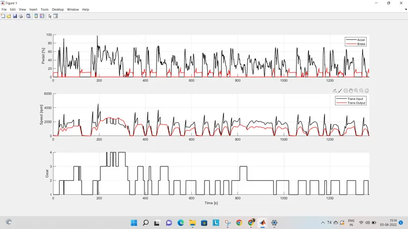
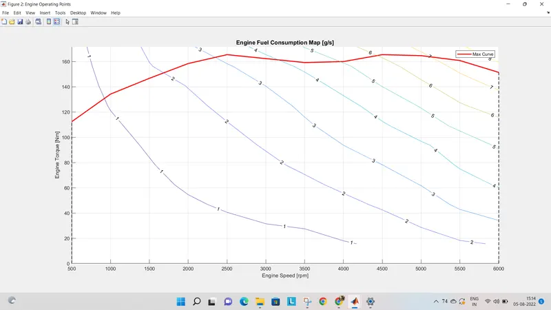
In this graph the plots for the acceleration pedal and the brake pedal are plotted. When we compared these plots to the previous plot that is with our UDDS drive cycle. that acceleration is higher in between the time range of 200 to 300 seconds again when we look into the graph of acceleration pedal and brake pedal we can experience the same heights in the acceleration padel between the period of 200 to 300th seconds and when the vehicle is accelerated between these time period we can see the brake pedal the value remains ZERO.And hence its very clear that the brake pedal values are zero, whenever there is a accleration. (ie., our vehicle is in running mode). Similarly you can see that the gear values are changing for various speeds.
For HWFET drive cycle:-
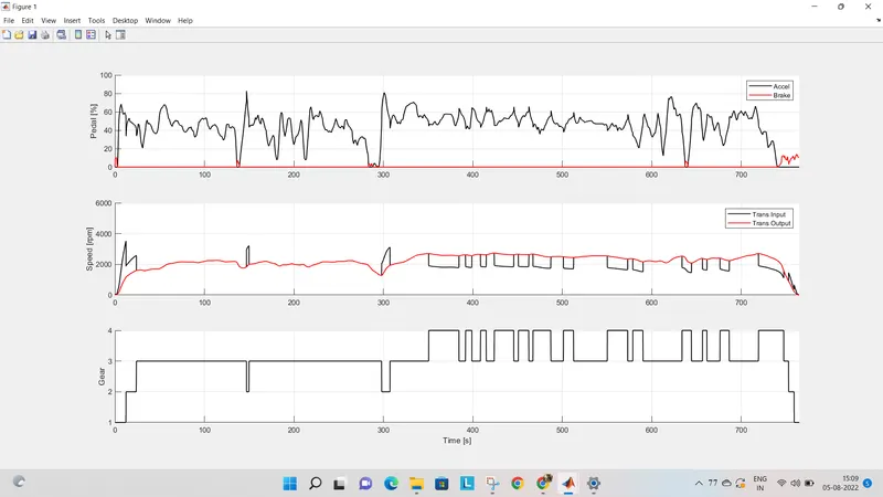
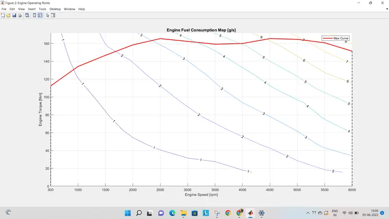
Here in this HWFET drive cycle, we can see that, almost most of the timme, the vehicle is in accleration and so we will see that the brake is used for very less time and the Gear is mostly maintined at 4.
NOTE:- THE MODIFIED .slx MODEL is attached with the Answer box