Project 1

AIM

Development of a forward energy-based fuel consumption model of a conventional vehicle.

Introduction

Conventional vehicle means any self-propelled, motorized vehicle designed for transporting persons or property on a public highway and must be registered. Conventional vehicles use an internal combustion engine works by fossil fuels. An internal combustion engine (ICE or IC engine) is a heat engine in which the combustion of a fuel occurs with an oxidizer (usually air) in a combustion chamber that is an integral part of the working fluid flow circuit. In an internal combustion engine, the expansion of the high-temperature and high-pressure gases produced by combustion applies direct force to some component of the engine.

The term internal combustion engine usually refers to an engine in which combustion is intermittent, such as the more familiar four-stroke and two-stroke piston engines, along with variants, such as the six-stroke piston engine and the Wankel rotary engine. ICEs are typically powered by fossil fuels like natural gas or petroleum products such as gasoline, diesel fuel or fuel oil. Renewable fuels like biodiesel are used in compression ignition (CI) engines

ENERGY AND PERFORMANCE OF THE VEHICLE

In this system the power demand on the wheel need to instant supplied by the powertrain. We can say that the power coming from the powertrain direct the power demand on the wheel

In this vehicle can be divided into 3 blocks Driver Block, Controller Unit, Powertrain.

The driver block gives the input to the vehicle and the controller act as the brain of the system and coordinate the input signal and control signal and give output on the wheel. In the powertrain it consists of engine transmission differential and wheel.

The engine generate power by converting chemical energy stored into the mechanical energy by the process of combustion. This has an efficiency and the energy input is in the form of fuel consumption.

Ie. Instantaneous Fuel Consumption

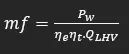
Where mf = mass flow rate in kg

Pw=Power on wheel.

myue=efficiency of engine.

myut=efficiency of transmission.

QLHV= calorific value of fuel

Energy Based Models- Element Models

To models the internal physical properties of the element and the losses there are basically two kinds of approach.

1)Map Based Model: - Elements are modelled using map which characterized the relationship between the input, output, losses etc.

2)Analytical Models: - Elements are modelled using physical equation that represent the internal dynamics.

These are two extreme most models that are the combination of two with some dynamics model analytically and using some maps

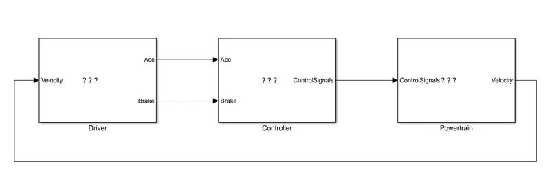
Here we use Forward model, which is known as the dynamic stimulation. Dynamic models are used for the detailed stimulation. Force, torque, power is the input and the state variable such as acceleration and velocity as the output. The models and stimulations are more realistic, a feedback loop to meet the desired vehicle state> It is mainly used to stimulate a vehicle on a driving cycle to analyse the dynamic behaviour of the system helps significantly in control development.

MATLAB CODE- INITIAL PREOCCESING CODE

RUN THE PROGRAM AND GIVE INPUT TO SIMULINK

%%%%%%%%%%%%%%%%%%%%%%%%%%%%%%%%%%%%%%%%%%%%%%%%%%%%%%%%%%%%%%%%%%%%%
%% Skill-Lync -> Hybrid Drives Development
% Project 1 - Conventional Vehicle Model
% By - Ullekh Gambhira 

% Description:

%% Initialization File
% Initialization file for loading the variables for the Conventional vehicle simulation model

%% Vehicle Parameters
M = 1500;       % Vehicle weight [kg]
Cr = 0.015;     % Rolling resistance coefficient
Rw = 0.35;      % Rolling radius [m]
Cd = 0.33;      % Drag coefficient
Af = 2;         % Frontal area [m2]
rhoa = 1.225;   % Air density [kg/m3]
Vwind = 0;      % Wind velocity [kmph]
g = 9.81;       % Gravitational acceleration [m/s2]
theta = 0;      % Slope [deg]
myu_road_tire = 1; % Coefficient of friction between tire - road interface

%% Powertrain Parameters 
FDR = 3.73;                         % Final Drive Ratio / Diff Ratio
DiffEff = 0.99;                     % Differential efficiency (assumed independent of operating conditions)

NumGear = 4;                        % Number of gears in transmission
TransGear = 1:NumGear;            % Transmission Gears
TransRatio = [3.06, 1.62, 1, 0.7];  % Corresponding Transmission ratios
TransEff = 0.90;                    % Transmission efficiency (assumed independent of operating conditions)

TC_SR = [0, .5, .6, .7, .8, .87, .92, .94, .96, .97, 1];   % Torque Converter Speed Ratio (Matlab default) -> TurbSpd/PumpSpd  
TC_TR = [2.232, 1.5462, 1.4058, 1.2746, 1.1528, 1.0732, 1.0192, 1, 1, 1, 1];   % Torque Converter Torque Ratio (Matlab default) -> TurbTrq/PumpTrq
TC_Cf = 1e-4 * [.72558, .66322, .63463, .59042, .51331, .4144, .29287, .22444, .12186, .04386, 0]; % Torque Converter Capacity Factor (Matlab default) -> PumpTrq/PumpSpd^2 [Nm/rpm^2]

load Vehicle_Data/Engine_data_1_9L_Saturn_95kW
load Vehicle_Data/Trans_Shift_map

%% Driver Parameters
Kp = 10;                    % P gain for driver PI model
Ki = 1;                     % I gain for driver PI model
Drive_Cycle_Select = 1;     % Drive cycle selection

% Drive cycle values in m/s

if Drive_Cycle_Select == 1
    load DriveCycles/UDDS;
    
elseif Drive_Cycle_Select == 2
    load DriveCycles/HWFET;
    
elseif Drive_Cycle_Select == 3
    load DriveCycles/FTP;
    
elseif Drive_Cycle_Select == 4
    load DriveCycles/US06;
    
elseif Drive_Cycle_Select == 5
    load DriveCycles/NEDC;
    
elseif Drive_Cycle_Select == 6
    load DriveCycles/WLTP;
 
end

time_end = cyc_time(end);
vel_end = cyc_vel(end);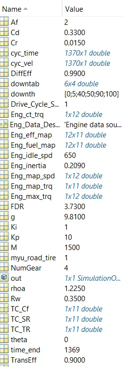

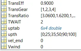
After that the physical modeling is take place using simulink open simulink and load the project processing file

In this project, a typical midsize car with a 1.9L engine and a 4-speed automatic transmission is considered. Data is taken from ADVISOR data base developed by NREL, USA. Transmission shift map and controller is taken from Matlab/Simulink example database.

The model developed has the capability to simulate the vehicle on different drive cycles like UDDS, HWFET, FTP, NEDC, etc.

“Project1_InitFile.m” is a Matlab script used to load all the variables required for running the Simulink model and for post-processing. The drive cycle selection is also done here. Before running the Simulink
vehicle model, run this initialization script.

Driver Block

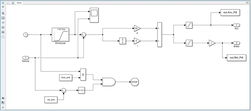
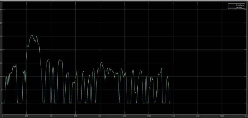
Driver Block is a basic PI controller that generate acceleration and brake pedal outputs to match the real velocity condition of a vehicle. It based on time, velocity then it all integrate and create output acceleration pedal and brake pedal.

Scope view

CONTROLLER BLOCK

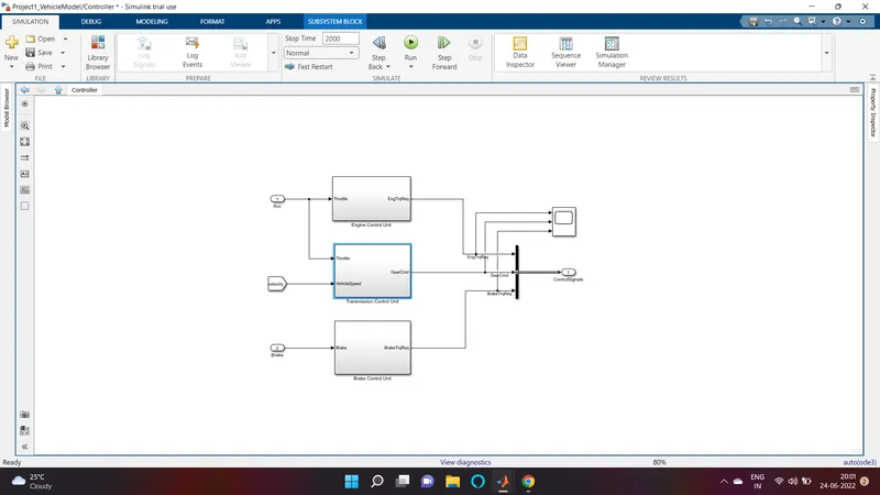
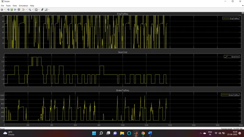
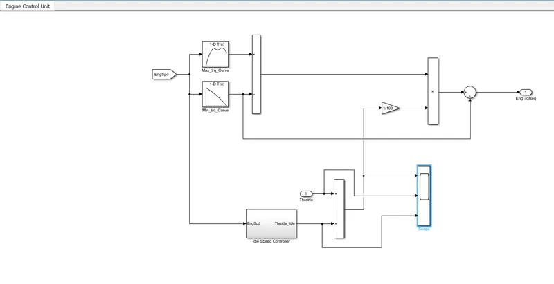
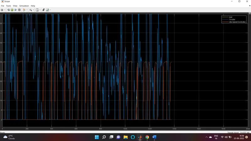
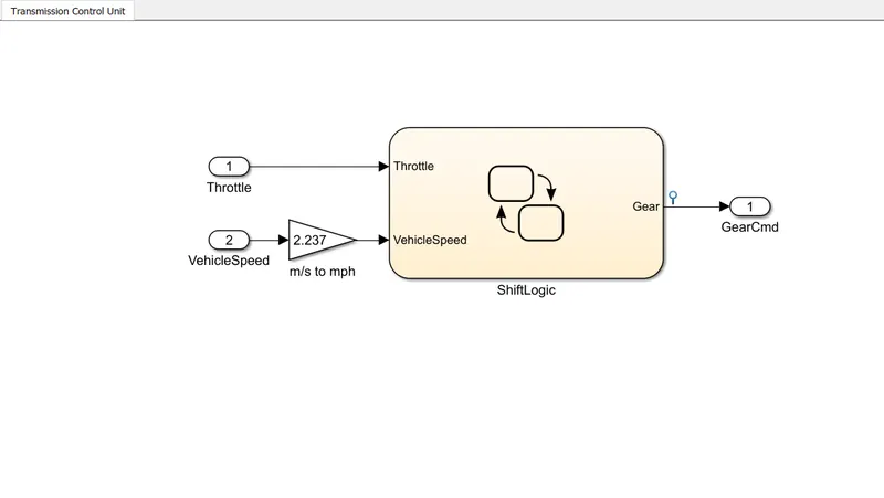
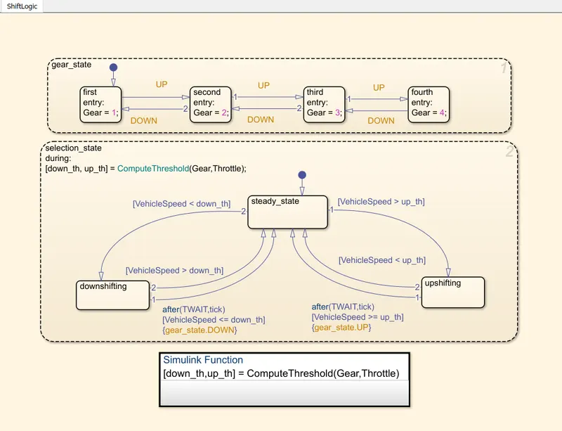
Controller block is a brain of the vehicle, representing the ECU (electronic control unit). Its is work according to the input given by the driver, it generates desired engine torque, transmission ratio, brake torque and give the signal to the powertrain.

SCOPE VIEW

ENGINE CONTROLL UNIT

TRANSMISSION CONTROLL UNIT

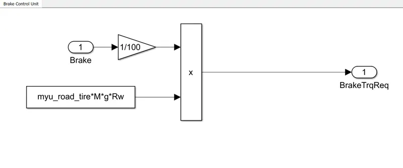
BRAKE CONTROLL UNIT

POWERTRAIN BLOCK

The movement component of the vehicle included in the powertrain. This includes as follows

1)ENGINE

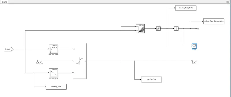
In engine block the fuel consumption of the engine is determining. It is based on maximum tourque and minimum torque from the controller and it saturated torque and give saturated torque and speed map give fuel consumption and then it get integrated.

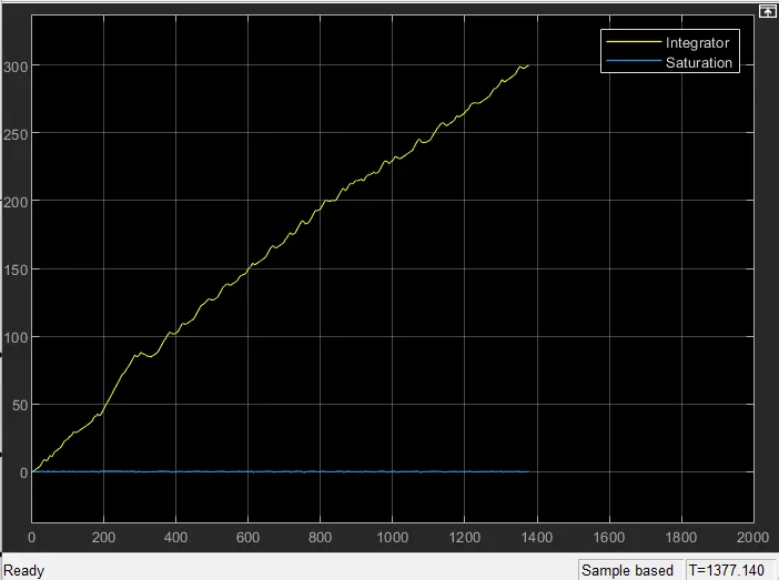
Scope view(UDDS)

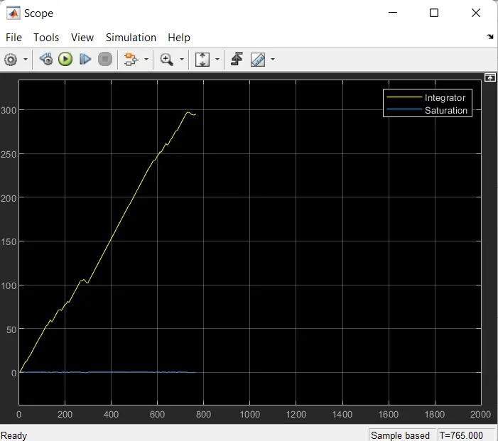
Scope view(HWFET)

2)TRANSMISSION BLOCK

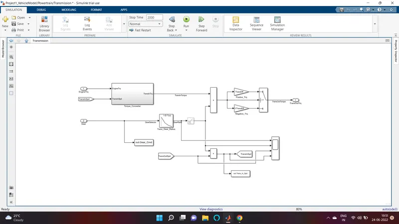
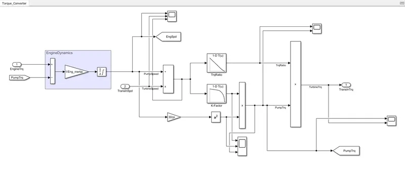
In transmission block the transmission gear ratio is determined according to the input engine torque, gear selector from the controller. The ratio is multiplied by the transmission input torque and then the transmission efficiency positive torque and negative torque gives transmission input speed. In this case torque convertor connects the engine to transmission and perform engine dynamic and decoupling.

Torque convertor block

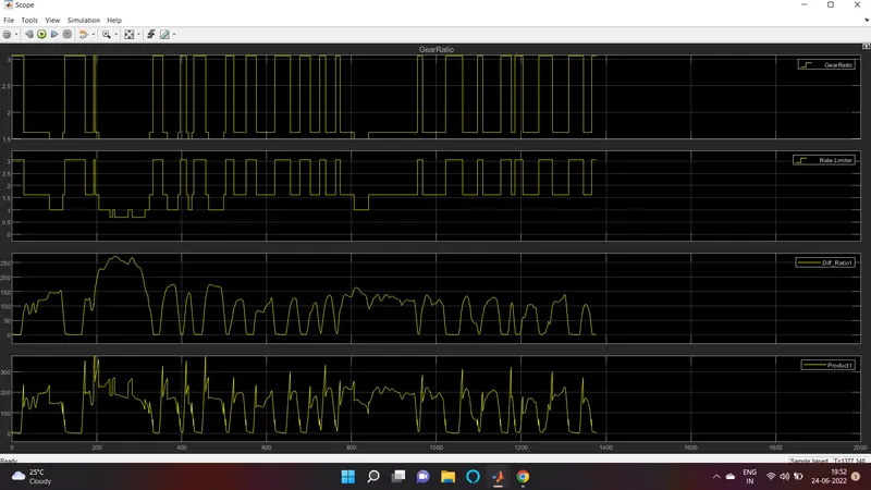
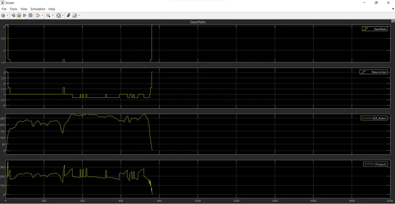
SCOPE VIEW-TRANSMISSION SPEED(IN/OUT)/GEAR RATIO/DIFFERENTIAL SPEED

UDDS

HWFET

DIFFERENTIAL BLOCK

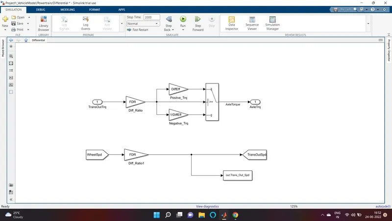
In differential block it takes input torque from the transmission and multiple the differential ratio and meet the axial torque. The axial torque is greater than the transmission torque and differential ratio.

WHEEL BLOCK

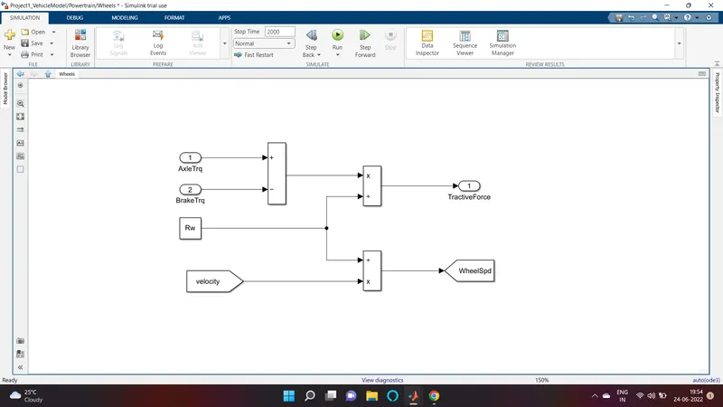
In wheel the axial torque from the differential and brake torque from the controller. It is subtracted and multiplied rolling radius and velocity then we met the tractive force from axle and brake torque and wheel speed.

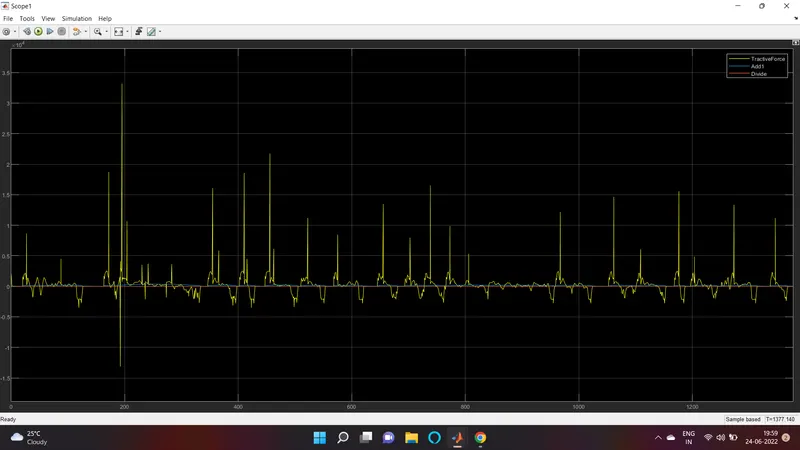
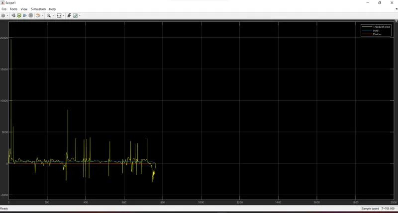
VEHICLE DYNAMICS

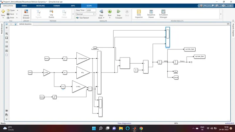
The powertrain power can be represented as follows,

Where is the force, is the tractional force on the wheel, is the drag force, is the rolling resistance force.

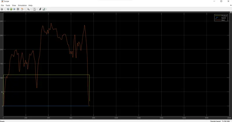
SCOPE VIEW-ROAD LOAD

USSD

HWFET

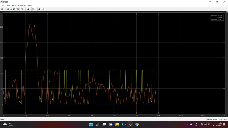
TRACTION FORCE/ROLLING RESISTANCE FORCE/DRAG RESISTANCE FORCE

UDDS

HWFET

AFTER RUNNING THE SIMULINK THEN RUN THE BELOW MATLAB SCRIPT

%%%%%%%%%%%%%%%%%%%%%%%%%%%%%%%%%%%%%%%%%%%%%%%%%%%%%%%%%%%%%%%%%%%%%
%% Skill-Lync -> Hybrid Drives Development
% Project 1 - Conventional Vehicle Model
% By - Ullekh Gambhira 

% Description:
% The following file is to used with the Initialization file and Simulink
% results for post-processing of the data.
% The file is incomplete, has some examples of how the data is imported
% into a readable format, data analysis and plotting examples.
% Based on the project task, use commands in a similar format as given
% below, to analyse the data and generate required plots.
% You can change variable names if desired

%% Post-Processing File
%  File for post-processing the Conventional vehicle simulation model data

%% Renaming variables
Time = out.tout;
Acc_Pdl = out.Acc_Pdl;          % Accelerator pedal [%]
Brk_Pdl = out.Brk_Pdl;          % Brake pedal [%]
Gear_Cmd = out.Gear_Cmd;        % Transmission gear
Trans_In_Spd = out.Trans_In_Spd*30/pi;  % Transmission input speed [rpm]
Trans_Out_Spd = out.Trans_Out_Spd*30/pi;% Transmission output speed [rpm]
Eng_Trq = out.Eng_Trq;          % Engine brake torque [Nm]
Eng_Spd = out.Eng_Spd*30/pi;    % Engine speed [rpm]
Eng_Fuel_Consump = out.Eng_Fuel_Consumption;    % Engine fuel consumption [g]
Veh_Dist = out.Veh_Dist/1000;   % Distance traveled by vehicle [km]
Veh_Spd = out.Veh_Spd*18/5;     % Vehicle speed [kmph]


%% Data Analysis
Eng_Pwr = Eng_Spd.*pi/30.*Eng_Trq/1000;   % Engine brake power [kW]
rho_petrol = 0.7197;                    % Density of petrol [kg/L]
kmpl = Veh_Dist(end)/(Eng_Fuel_Consump(end)/1000/rho_petrol);    % Fuel economy [kmpl] 


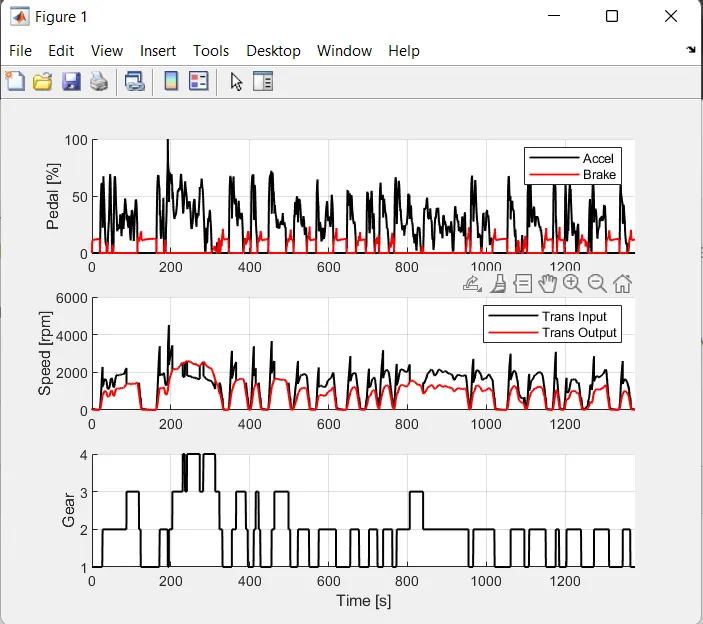
%% Plotting vehicle characteristics time trace
figure(1)
subplot(3,1,1)
hold on
grid on
plot(Time, Acc_Pdl, 'linewidth', 1, 'Color', 'black');
plot(Time, Brk_Pdl, 'linewidth', 1, 'Color', 'red');
ylabel('Pedal [%]')
xlim([0, Time(end)]);
legend('Accel','Brake');
subplot(3,1,2)
hold on
grid on
plot(Time, Trans_In_Spd, 'linewidth', 1, 'Color', 'black');
plot(Time, Trans_Out_Spd, 'linewidth', 1, 'Color', 'red');
ylabel('Speed [rpm]')
xlim([0, Time(end)]);
ylim([0, 6000]);
legend('Trans Input','Trans Output');
subplot(3,1,3)
hold on
grid on
plot(Time, Gear_Cmd, 'linewidth', 1, 'Color', 'black');
xlim([0, Time(end)]);
xlabel('Time [s]');
ylabel('Gear');
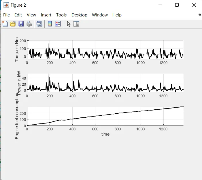
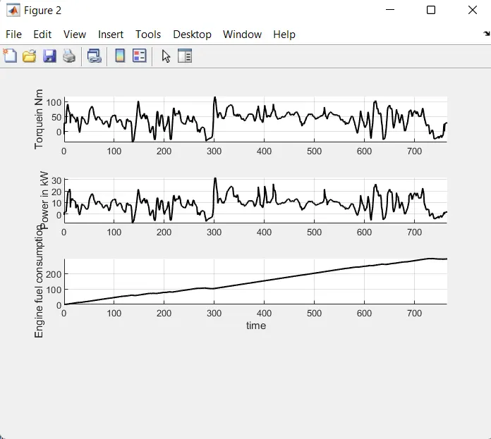
%% plotting engine torque, engine power, fuel rate and fuel consumption
figure(2)
subplot(4,1,1)
hold on
grid on
plot(Time, Eng_Trq, 'linewidth', 1, 'Color', 'black');
ylabel('Torquein Nm');
xlim([0,Time(end)]);
subplot(4,1,2)
hold on
grid on
plot(Time, Eng_Pwr, 'linewidth', 1, 'Color', 'black');
ylabel('Power in kW');
xlim([0,Time(end)]);
subplot(4,1,3)
hold on
grid on
plot(Time, Eng_Fuel_Consump, 'linewidth', 1, 'Color', 'black');
xlabel('time')
ylabel('Engine fuel consumption');
xlim([0,Time(end)]);
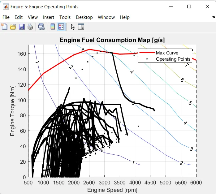
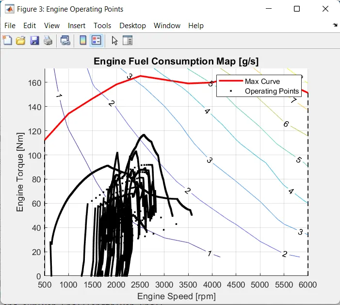
%% Plotting engine operating points on engine fuel map
figure('Name','Engine Operating Points');
hold on
grid on
title('Engine Operating Points','fontsize',12);
p1=plot(Eng_map_spd*30/pi,Eng_max_trq,'linewidth',2,'color','r');
p2=line([Eng_map_spd(end)*30/pi Eng_map_spd(end)*30/pi],[0 Eng_max_trq(end)]);
set(p2,'linewidth',1,'linestyle','--','color','k');
p3=line([Eng_map_spd(1)*30/pi Eng_map_spd(1)*30/pi],[0 Eng_max_trq(1)]);
set(p3,'linewidth',1,'linestyle','--','color','k');
[c,h] = contour(Eng_map_spd'*30/pi,Eng_map_trq,Eng_fuel_map');
clabel(c,h);
xlabel('Engine Speed [rpm]');
ylabel('Engine Torque [Nm]');
title('Engine Fuel Consumption Map [g/s]');
p4 = plot(Eng_Spd,Eng_Trq,'.','color','k');
legend([p1 p4],{'Max Curve','Operating Points'});
axis([Eng_map_spd(1)*30/pi Eng_map_spd(end)*30/pi 0 Eng_map_trq(end)]);


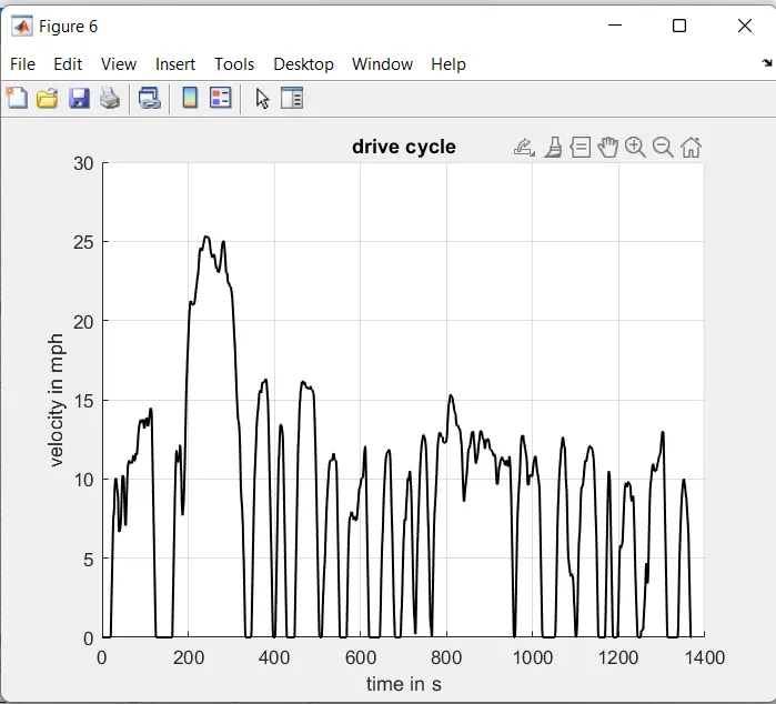
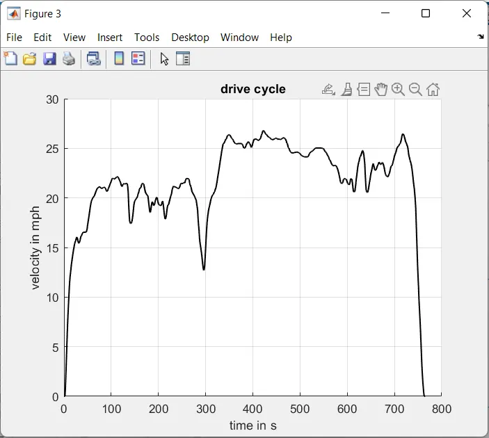
%% plottting drive cycle
figure()
hold on
grid on
plot(cyc_time, cyc_vel,'LineWidth',1,'Color','black')
xlabel('time in s')
ylabel('velocity in mph')
title('drive cycle')
%% test result
avg_spd=sum(Veh_Spd)/length(Veh_Spd);
max_spd=maxk(Veh_Spd,1);
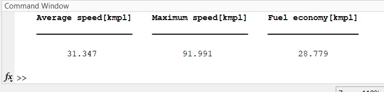
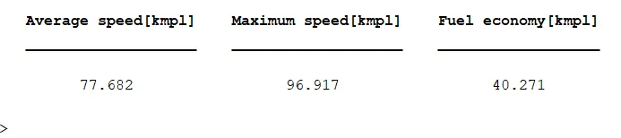
table(avg_spd,max_spd,kmpl,'VariableNames',{'Average speed[kmpl]','Maximum speed[kmpl]','Fuel economy[kmpl]'})

RESULT for UDDS

torque/power/fuel consumption

RESULT FOR HWFET

torque/power/fuel consumption

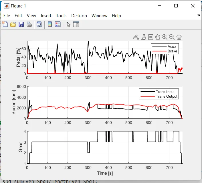
OBSERVATIONS

1) The fuel economy of urban drive is much lower than the highway drive

2) The torque demand of the drive cycle are different, so the fuel flow rate varies and fuel consumption is calculated.

3) The HWFET drive cycle has higher power and torque requirmnt and less negative torque and power. it because brake requrment are low ,more accelerator pedal are used and smooth drive is possible

4)In fuel map the engine operating points are plotted and the operating point is under the maximum torque curve.

CONCLUSION

Hence,development of a forward energy-based fuel consumption model of a conventional vehicle has been successfully stimulated using Matlab and Simulink.

Engine speed, torque, transmission speed, gear and distance travelled are traced and analyasis

Required plots and graphs are plotted using the post process calculation.

Able to calculated the kmpl and drive cycle such as UDDS and HWFET.