Data cleaning and Descriptive analytics on the Automobile 1985 dataset

Aim :

To perform data cleaning and descriptive analytics on the Automobile 1985 dataset

Dataset :

The dataset is about cars from 1985, It consists of:

Number of Instances: 205

Number of Attributes: 26 total

• 15 continuous
• 1 integer
• 10 nominal

Methods :

Data cleaning

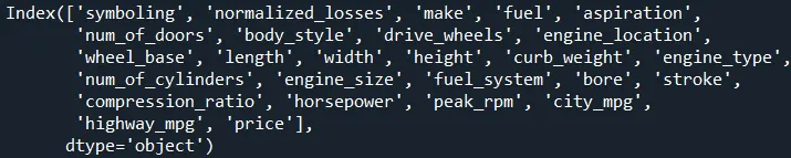
The dataset is read using pandas and the column names are assigned for each attribute, The column names are as follows

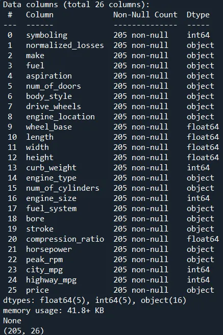
The info and shape of the dataset are

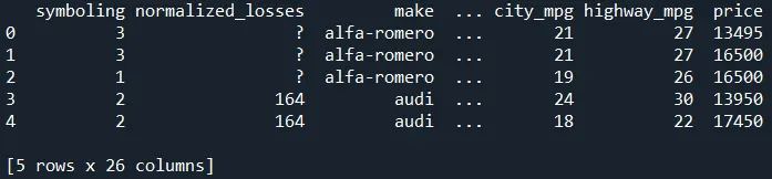
The first 5 records of the dataset

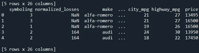
'?' implies an empty value so we change '?' to NAN

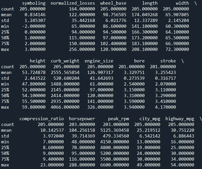
Changing the data type of the attributes to see the mean, standard deviation, max, etc.

Checking for the total number of empty values

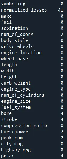
Now we replace empty values with mean for attributes like normalized_losses, bore, stroke, horsepower, and peak_rpm. For the number of doors, we substitute the most frequent value since it is a categorical data mean would not make sense. Also for the price, we drop the records with empty values.

Feature engineering

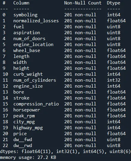
We change the categorical data into numerical using one-hot encoding and drop the features which are not required.

We plot a correlation matrix to find highly correlated features and drop those features

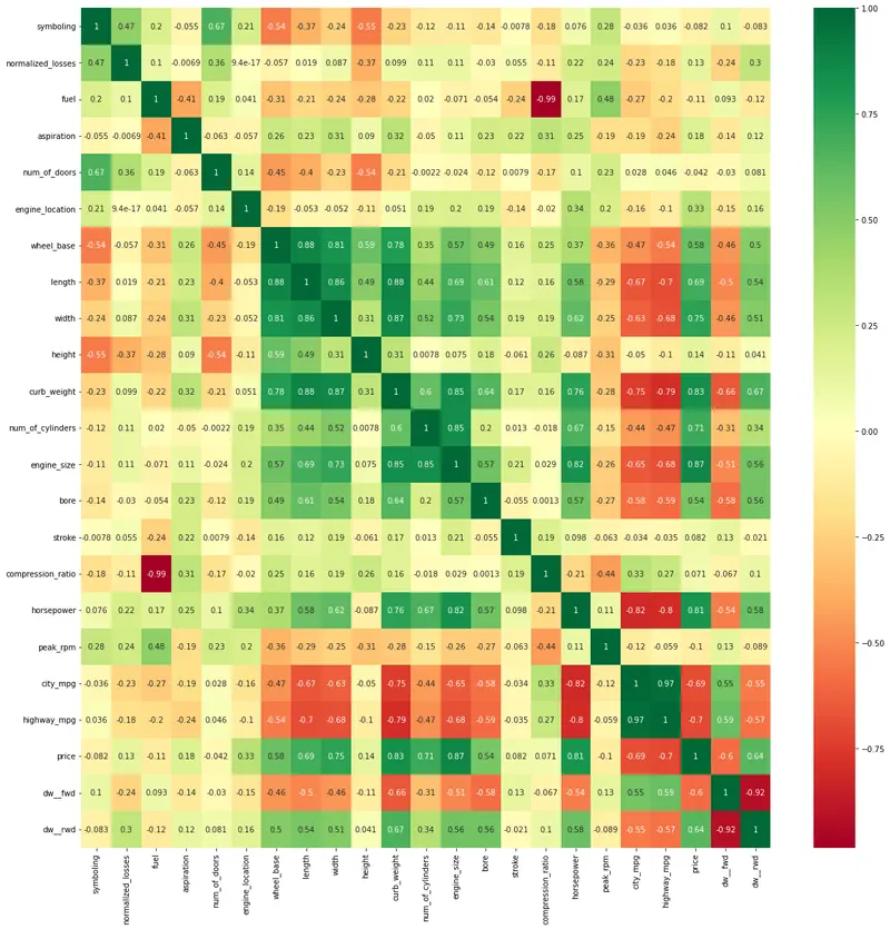
Highway_mpg and compression_ratio are dropped.

Using standard scaler the whole data set is standardized

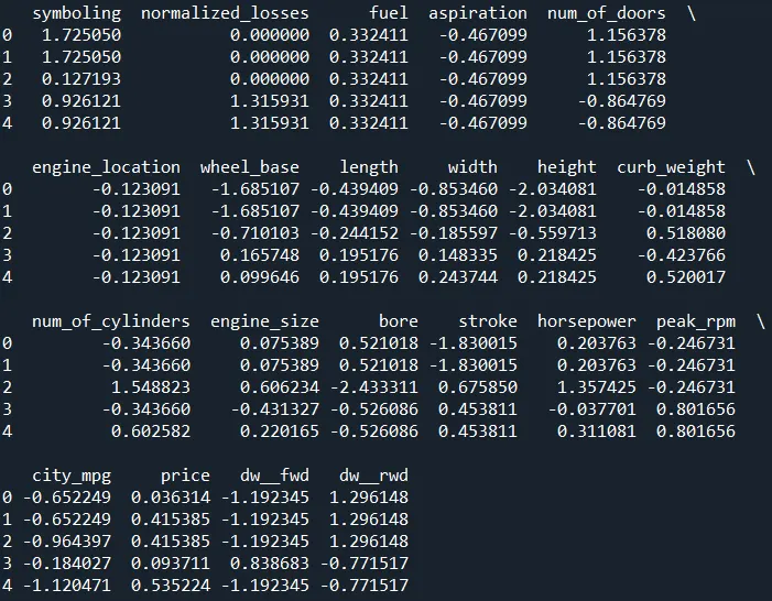
Exploratory data analysis

Box plots for different features and prices were plotted

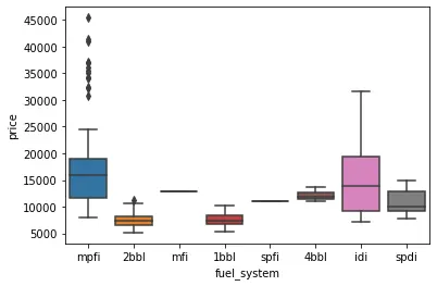
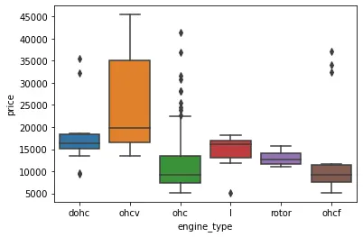
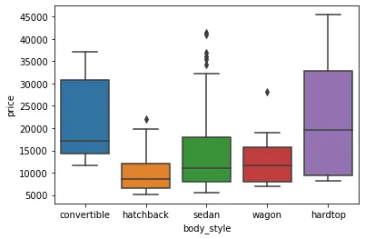
As we can see body_style, engine_type and fuel_system do not vary much with price hence these features are dropped

Scatter plots are used to find which features can be used to predict the price of the cars

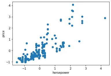
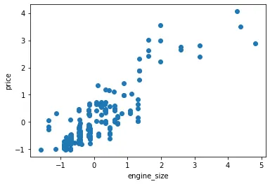
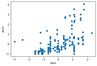
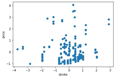
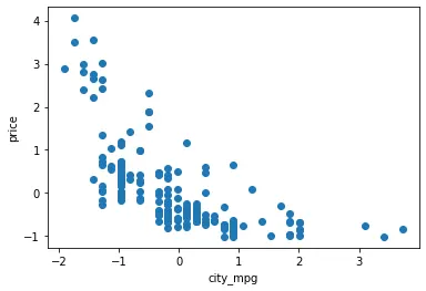
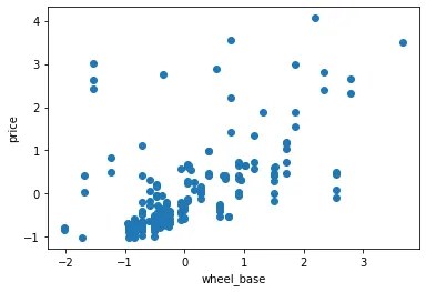
Horsepower and engine_size are very well predictors of price of the cars

Code :

import pandas as pd
import numpy as np
import matplotlib.pyplot as plt
import seaborn as sns
from sklearn.preprocessing import StandardScaler

#Assign names to each column
column_name=['symboling','normalized_losses','make','fuel','aspiration','num_of_doors','body_style','drive_wheels','engine_location','wheel_base','length','width','height','curb_weight','engine_type','num_of_cylinders','engine_size','fuel_system','bore','stroke','compression_ratio','horsepower','peak_rpm','city_mpg','highway_mpg','price']

#Read dataset
df=pd.read_csv('auto.csv',names = column_name)
print(df.columns)

print(df.info())
print(df.shape)
print(df.head())

# Replacing ? with NAN
df.replace("?",np.nan,inplace=True)
print(df.head())

#Converting datatype
#pd.set_option('display.max_columns', None)
df['normalized_losses']=df['normalized_losses'].astype(float)
df['bore']=df['bore'].astype(float)
df['stroke']=df['stroke'].astype(float)
df['horsepower']=df['horsepower'].astype(float)
df['peak_rpm']=df['peak_rpm'].astype(float)
df['price']=df['price'].astype(float)

print(df.describe())

#Finding total null values
print(df.isna().sum())

#Dealing with null values

#Replacing with mean values
df['normalized_losses'].replace(np.nan, 122,inplace=True)
df['bore'].replace(np.nan, 3.329050,inplace=True)
df['stroke'].replace(np.nan, 3.258300,inplace=True)
df['horsepower'].replace(np.nan, 104.222772,inplace=True)
df['peak_rpm'].replace(np.nan, 5125.990099,inplace=True)

#Replacing with highest frequency values
print(df['num_of_doors'].value_counts())
df['num_of_doors'].replace(np.nan, 'four',inplace=True)

#Dropping values
df.dropna(subset=["price"], axis=0, inplace=True)
df.reset_index(drop=True, inplace=True)
print(df.head())


#Feature engineering
df['fuel']=pd.get_dummies(df['fuel'],drop_first=True)

df['aspiration']=pd.get_dummies(df['aspiration'],drop_first=True)

df['num_of_doors']=pd.get_dummies(df['num_of_doors'],drop_first=True)

df['engine_location']=pd.get_dummies(df['engine_location'],drop_first=True)

df['num_of_cylinders'].replace('two', 2,inplace=True)
df['num_of_cylinders'].replace('three', 3,inplace=True)
df['num_of_cylinders'].replace('four', 4,inplace=True)
df['num_of_cylinders'].replace('five', 5,inplace=True)
df['num_of_cylinders'].replace('six', 6,inplace=True)
df['num_of_cylinders'].replace('eight', 8,inplace=True)
df['num_of_cylinders'].replace('twelve', 12,inplace=True)
df['num_of_cylinders']=df['num_of_cylinders'].astype(int)

gd = pd.get_dummies(df['drive_wheels'], prefix='dw_',drop_first=True)
df = pd.merge(left=df,right=gd,left_index=True,right_index=True)

#sns.boxplot(x="body_style", y="price", data=df)
#sns.boxplot(x="engine_type", y="price", data=df)
#sns.boxplot(x="fuel_system", y="price", data=df)

#Dropping unwanted features
df=df.drop(['make','drive_wheels','engine_type','fuel_system','body_style'],axis=1)
print(df.info())


#Corelation matrix
corr=df.corr().index
#plt.figure(figsize=(20,20))
#sns.heatmap(df[corr].corr(),annot=True,cmap='RdYlGn')

#Dropping highly corelated features
df=df.drop(['highway_mpg','compression_ratio'],axis=1)
print(df.info())
print(df.shape)

#Standardizing the data
sc=StandardScaler()
df=sc.fit_transform(df)
column_name2=['symboling','normalized_losses','fuel','aspiration','num_of_doors','engine_location','wheel_base','length','width','height','curb_weight','num_of_cylinders','engine_size','bore','stroke','horsepower','peak_rpm','city_mpg','price','dw__fwd','dw__rwd']
df=pd.DataFrame(df)
df.columns=column_name2
print(df.head())
plt.scatter(df['wheel_base'],df['price'])
plt.xlabel('wheel_base')
plt.ylabel('price')