Project 1

AIM

To study the forward energy-based fuel consumption model of a conventional vehicle.

OBJECTIVE

• To run the model, determine the calculations and generate plots for both Urban cycle (UDDS) and highway cycle (HWFET).
• Analyze and understand the vehicle operating points in terms of engine speed, torque, transmission speeds, pedal positions, gear, distance traveled, etc.
• Complete the engine and vehicle dynamics block contents, which have been detected from the model.
• Modify the “ Project1_ProcessingFile.m” as per the desired plots and required calculations.

THEORY

FORWARD ENERGY-BASED FUEL CONSUMPTION MODEL OF A CONVENTIONAL VEHICLE

• It is the forward model, that is model and simulation are more realistic due to physical causality, hence appropriate for control development and there is a feedback loop to meet the desired vehicle state.
• It is based on fuel consumption. The model is convenient for analyzing and understanding the vehicle traveled with how much fuel is consumed according to different drive cycles. That will realize the vehicle performance and conclude the optimal usage.
• In this project, a typical mid-size car with a 1.9L engine and a 4- speed automatic transmission is considered. Data is taken from the ADVISOR database developed by NREL, USA. The transmission shift map and controller are taken from Matlab/Simulink example database.
• Here three files are needed to run. The first one is initializing the script (Project1_initFile.m) with variables required for running the Simulink model. The second one is a post-processing script (Project1_ProcessingFile.m) with required calculations and commands for generating desired plots.
• The third one is the Simulink model (Project1_vehicleModel.slx). It is modeled using a ‘Driver’ block, which is a basic PI controller that generates accelerator and brake pedal outputs to match the desired and actual vehicle speeds. The ‘Controller’ block is the brain of the vehicle, representing the electronic controls units. Based on the driver inputs, it generates desired engine torque, desired transmission gear
  and desired brake torque. These inputs are fed to the ‘Powertrain’ block which represents the drivetrain of the vehicle. It consists of an ‘Engine’ connected to the ‘Automatic Transmission’ through a ‘Torque Converter’. The output of the transmission is connected to the ’Differential’, which powers the ‘Wheels’, which provide the tractive force for vehicle acceleration. The longitudinal dynamics of the vehicle along with the road load are represented in the ‘Vehicle Dynamics’ block.

Drive Cycles

• A drive cycle is a series of trips, usually one or two, theta vehicle is required to undergo. Here two drive cycles are used. The first one is the Urban dynamometer driving schedule (UDDS), which represents city/ urban driving conditions, where a vehicle is started with the engine cold and driven in stop and go busy traffic. It is used for light-duty vehicle testing and max speed of 56 mph.
• The second one is highway fuel economy driving schedule (HWFET), which represents a mixture of rural and interstate highway driving with a warmed- up-engine, typical for longer trips in free-flowing traffic and a max speed of 60mph.

EQUATIONS INVOLVED

Engine Power (kW) =`(πNT)/(30×1000)`

Where, N = engine speed in rpm

T = engine torque in Nm

Fuel Ecnomy, Kmpl =`(dist)/(fuel cons)`

Where, dist = distance traveled by vehicle

Fuel cons = Fuel consumed in L

INITIAL SCRIPT

%%%%%%%%%%%%%%%%%%%%%%%%%%%%%%%%%%%%%%%%%%%%%%%%%%%%%%%%%%%%%%%%%%%%%
%% Skill-Lync -> Hybrid Drives Development
% Project 1 - Conventional Vehicle Model
% By - Ullekh Gambhira 

% Description:

%% Initialization File
% Initialization file for loading the variables for the Conventional vehicle simulation model

%% Vehicle Parameters
M = 1500;       % Vehicle weight [kg]
Cr = 0.015;     % Rolling resistance coefficient
Rw = 0.35;      % Rolling radius [m]
Cd = 0.33;      % Drag coefficient
Af = 2;         % Frontal area [m2]
rhoa = 1.225;   % Air density [kg/m3]
Vwind = 0;      % Wind velocity [kmph]
g = 9.81;       % Gravitational acceleration [m/s2]
theta = 0;      % Slope [deg]
myu_road_tire = 1; % Coefficient of friction between tire - road interface

%% Powertrain Parameters 
FDR = 3.73;                         % Final Drive Ratio / Diff Ratio
DiffEff = 0.99;                     % Differential efficiency (assumed independent of operating conditions)

NumGear = 4;                        % Number of gears in transmission
TransGear = [1:NumGear];            % Transmission Gears
TransRatio = [3.06, 1.62, 1, 0.7];  % Corresponding Transmission ratios
TransEff = 0.90;                    % Transmission efficiency (assumed independent of operating conditions)

TC_SR = [0, .5, .6, .7, .8, .87, .92, .94, .96, .97, 1];   % Torque Converter Speed Ratio (Matlab default) -> TurbSpd/PumpSpd  
TC_TR = [2.232, 1.5462, 1.4058, 1.2746, 1.1528, 1.0732, 1.0192, 1, 1, 1, 1];   % Torque Converter Torque Ratio (Matlab default) -> TurbTrq/PumpTrq
TC_Cf = 1e-4 * [.72558, .66322, .63463, .59042, .51331, .4144, .29287, .22444, .12186, .04386, 0]; % Torque Converter Capacity Factor (Matlab default) -> PumpTrq/PumpSpd^2 [Nm/rpm^2]

load Vehicle_Data/Engine_data_1_9L_Saturn_95kW
load Vehicle_Data/Trans_Shift_map

%% Driver Parameters
Kp = 10;                    % P gain for driver PI model
Ki = 1;                     % I gain for driver PI model
Drive_Cycle_Select = 2;     % Drive cycle selection

% Drive cycle values in m/s

if Drive_Cycle_Select == 1
    load DriveCycles/UDDS;
    
elseif Drive_Cycle_Select == 2
    load DriveCycles/HWFET;
    
elseif Drive_Cycle_Select == 3
    load DriveCycles/FTP;
    
elseif Drive_Cycle_Select == 4
    load DriveCycles/US06;
    
elseif Drive_Cycle_Select == 5
    load DriveCycles/NEDC;
    
elseif Drive_Cycle_Select == 6
    load DriveCycles/WLTP;
 
end

time_end = cyc_time(end);
vel_end = cyc_vel(end);

POST PROCESSING SCRIPT

%%%%%%%%%%%%%%%%%%%%%%%%%%%%%%%%%%%%%%%%%%%%%%%%%%%%%%%%%%%%%%%%%%%%%
%% Skill-Lync -> Hybrid Drives Development
% Project 1 - Conventional Vehicle Model
% By - Ullekh Gambhira 

% Description:
% The following file is to used with the Initialization file and Simulink
% results for post-processing of the data.
% The file is incomplete, has some examples of how the data is imported
% into a readable format, data analysis and plotting examples.
% Based on the project task, use commands in a similar format as given
% below, to analyse the data and generate required plots.
% You can change variable names if desired

%% Post-Processing File
%  File for post-processing the Conventional vehicle simulation model data

%% Renaming variables
Time = out.tout;
Acc_Pdl = out.Acc_Pdl;          % Accelerator pedal [%]
Brk_Pdl = out.Brk_Pdl;          % Brake pedal [%]
Gear_Cmd = out.Gear_Cmd;        % Transmission gear
Trans_In_Spd = out.Trans_In_Spd*30/pi;  % Transmission input speed [rpm]
Trans_Out_Spd = out.Trans_Out_Spd*30/pi;% Transmission output speed [rpm]
Eng_Trq = out.Eng_Trq;          % Engine brake torque [Nm]
Eng_Spd = out.Eng_Spd*30/pi;    % Engine speed [rpm]
Eng_Fuel_Consump = out.Eng_Fuel_Consumption;    % Engine fuel consumption [g]
Veh_Dist = out.Veh_Dist/1000;   % Distance traveled by vehicle [km]
Veh_Spd = out.Veh_Spd*18/5;     % Vehicle speed [kmph]
Eng_Fuel_Rate = out.Eng_Fuel_Rate; % Engine fuel rate [g/s]
Whl_Spd = out.Whl_Spd*30/pi;    % wheel speed [rpm]
Dsr_Spd = out.Dsr_Spd*18/5;     % desired vehicle speed [kmph]

%% Data Analysis
Eng_Pwr = Eng_Spd*(pi/30).*Eng_Trq/1000;   % Engine brake power [kW]
rho_petrol = 0.7197;                       % Density of petrol [kg/L]
 kmpl = Veh_Dist(end)/(Eng_Fuel_Consump(end)/(1000*rho_petrol));    % Fuel economy [kmpl] 


%% Plotting vehicle characteristics time trace for engine, transmission input, transmission output and wheel speed on one plot
figure()
hold on 
grid on 
plot(Time,Eng_Spd,'color','r')
plot(Time,Trans_In_Spd,'color','y')
plot(Time,Trans_Out_Spd,'color','k')
plot(Time,Whl_Spd,'color','g')
ylabel('speeds [rpm]')
xlabel('Time [s]')
xlim([0,Time(end)])
legend('engine speed','trans in spd','trans out spd','wheel spd')

%% engine torque, engine power, fuel rate and consumption using subplots
figure()
subplot(4,1,1)
hold on
grid on
plot(Time,Eng_Trq)
ylabel('engine torque [Nm]')
xlim([0,Time(end)])
subplot(4,1,2)
hold on
grid on
plot(Time,Eng_Pwr)
ylabel('engine power [kW]')
xlim([0,Time(end)])
subplot(4,1,3)
hold on
grid on
plot(Time,Eng_Fuel_Rate)
ylabel('engine fuel rate [g/s]')
xlim([0,Time(end)])
subplot(4,1,4)
hold on
grid on
plot(Time,Eng_Fuel_Consump)
ylabel('engine fuel consumption [g]')
xlabel('Time [s]')
xlim([0,Time(end)])

%% accelerator and brake pedal, gear command, vehicle desired and actual speed, vehicle distance using subplots
figure()
subplot(4,1,1)
hold on
grid on
plot(Time, Acc_Pdl, 'linewidth', 1, 'Color', 'black');
plot(Time, Brk_Pdl, 'linewidth', 1, 'Color', 'red');
ylabel('Pedal [%]')
xlim([0, Time(end)]);
legend('Accel','Brake');
subplot(4,1,2)
hold on
grid on
plot(Time, Gear_Cmd, 'linewidth', 1, 'Color', 'black');
xlim([0, Time(end)]);
ylabel('Gear')
subplot(4,1,3)
hold on
grid on
plot(Time, Veh_Spd, 'linewidth', 1, 'Color', 'black');
plot(Time, Dsr_Spd, 'linewidth', 1, 'Color', 'red');
ylabel('Speed [kmph]')
xlim([0,Time(end)]);
legend('Actual speed','Desired speed');
subplot(4,1,4)
hold on
grid on
plot(Time, Veh_Dist, 'linewidth', 1, 'Color', 'black');
ylabel(['distance [km]'])
xlim([0,Time(end)]);
xlabel('Time [s]')

%% Plotting engine operating points on engine fuel map
figure('Name','Engine Operating Points');
hold on
grid on
p1=plot(Eng_map_spd*30/pi,Eng_max_trq,'linewidth',2,'color','r');
p2=line([Eng_map_spd(end)*30/pi Eng_map_spd(end)*30/pi],[0 Eng_max_trq(end)]);
set(p2,'linewidth',1,'linestyle','--','color','k');
p3=line([Eng_map_spd(1)*30/pi Eng_map_spd(1)*30/pi],[0 Eng_max_trq(1)]);
set(p3,'linewidth',1,'linestyle','--','color','k');
[c,h] = contour(Eng_map_spd'*30/pi,Eng_map_trq,Eng_fuel_map');
clabel(c,h);
xlabel('Engine Speed [rpm]');
ylabel('Engine Torque [Nm]');
title('Operating Points in Engine Fuel Consumption Map','fontsize',12);
p4 = plot(Eng_Spd,Eng_Trq,'.','color','k');
legend([p1 p4],{'Max Curve','Operating Points'});
axis([Eng_map_spd(1)*30/pi Eng_map_spd(end)*30/pi 0 Eng_map_trq(end)]);

SIMULINK MODEL

click here for simulink model- google drive link

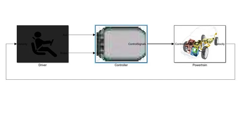
figure 1. vehicle model

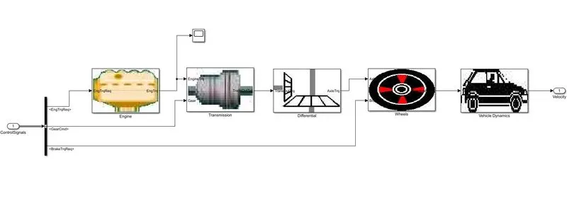
figure 2. power train subsystem inside

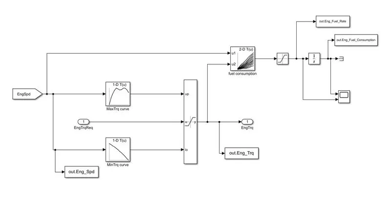
figure 3. completed engine block

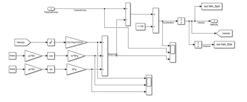
figure 4. completed vehicle dynamics block

RESULT

URBAN DYNAMOMETER DRIVING SCHEDULE (UDDS)

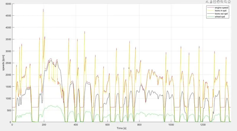
Figure 5. speed vs time

This graph gives the speed of the engine, transmission, and wheel concerning the cycle time. We can see that speed decreases from the engine to the wheel because of the transmission and differential losses.

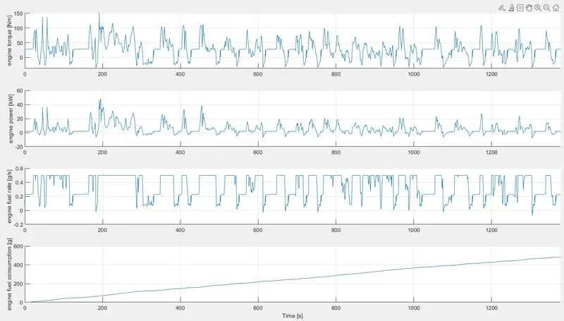
Figure 6. subplot

This is the subplot of engine torque, engine power, engine fuel rate, and engine fuel consumption.

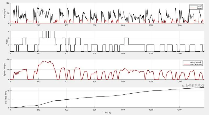
Figure 7. subplot

This is the subplot of acceleration and pedal movement, gear, vehicle speed, and distance.

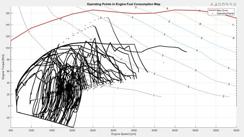
Figure 8. engine fuel consumption map

This is the engine fuel consumption map of where the operating points of engines are plotted.

• It is the urban drive cycle operation. Which represents city driving conditions. The vehicle is driving in stop-and-go busy traffic. That has shown in the figure. In figure 1, we can see the wheel speed of the vehicle. where wheel speed becomes zero when the vehicle stops. At vehicle stops then the transmission input, transmission output, and wheel speeds become zero and while engine speed does not go to zero. Because it’s a traffic block situation, in that short time the engine does not shut down. That’s why the engine keeps some speed at idle time. Where transmission disengages from the engine at the idle time and this leads to speeds of transmission input and output and the wheel becomes zero at idle time. We can also see the difference in speed between the components such as engine, and transmission input because the engine and transmission are connected with a torque converter, which is fluid coupling. This makes a slight difference in speed between engine and transmission input.
• The next figure gives the details regarding engine torque, engine power, engine fuel rate, and engine fuel consumption. The drive cycle is used which is UDDS. Idle time fuel consumption is need to consider because in this drive cycle having more idle time that’s because of stop and go traffic conditions. Engine power fluctuation is visible between 0 to 20kw in the majority. Large torque fluctuation can be seen because of stop and go conditions engine fuel consumption is beyond 400g at the end of drive cycle.
• The next figure having subplots of the pedal, gear, vehicle speed, and distance are generated. Here we can see the pedal position graph that shows how much percentage of each pedal is applied which is the acceleration pedal and the brake pedal. Which is applied. The gear position is also noted in the graph. Gear change between 1and 2 is more. Because stop and go traffic conditions. Vehicle speed is less than 50 kmph in the majority. Here the distance traveled is between 10-11 km.
• The next figure is the engine fuel consumption map where we can see that the operating point of the engine is plotted on this fuel consumption map. Operating points depend on pedal positions and gear. Which controls the speed and torque coming from the engine. In the case of which gear is using that provides different torque and speed. That is lower gears give more torque and medium speed and vice versa. According to this UDDS cycle has more stop-and-go driving conditions. This leads to gear shift being more between 1and 2. It can be seen that the majority of operating points are lying areas of medium torque and medium speed because of stop-and-go traffic conditions in the UDDS drive cycle.

HIGHWAY FUEL ECONOMY DRIVING SCHEDULE (HWFET)

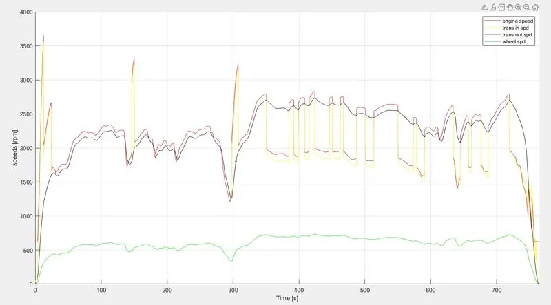
Figure 9. speed vs time

This graph gives the speed of the engine, transmission, and wheel concerning the cycle time. We can see that speed decreases from the engine to the wheel because of the transmission and differential losses.

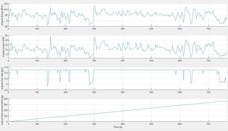
Figure 10. subplot

This is the subplot of engine torque, engine power, engine fuel rate, and engine fuel consumption.

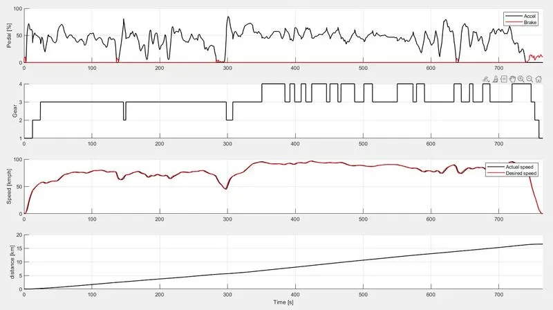
Figure 11. subplot

This is the subplot of acceleration and pedal movement, gear, vehicle speed, and distance.

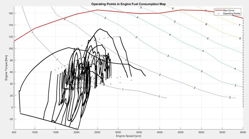
Figure 12. engine fuel consumption map

This is the engine fuel consumption map of where the operating points of engines are plotted.

• It is the highway fuel economy testing cycle operation. Which represents a mixture of rural and interstate highway driving and typical of longer trips in free-flowing traffic. That is shown in the figure. In figure1, we can see the speed of the engine, transmission, and wheel. Here engine speed is above 1500 rpm in the majority. Because it’s a highway’s nonstop conditions. That makes the vehicle moves at high speed. Engine and transmission input provide a slight difference in speed. Whereas transmission output speed has few differences compared to wheel speed.
• The next figure gives the details regarding engine torque, engine power, engine fuel rate, and engine fuel consumption. The drive cycle is used which is HWFET. There is no idle time fuel consumption because of having no idle time here. Engine power fluctuation can be seen from 0 to 40 kW in the majority. There are a few torque fluctuations that can be seen. Because of highway conditions, the engine fuel rate is constant most of the time and the fuel consumption is between 300 to 400g at the end of the drive cycle.
• The next figure having subplots of the pedal, gear, vehicle speed, and distance are generated. Here we can see that pedal position graph. The acceleration pedal is applied in the majority of the brake pedal because of nonstop highway conditions. The high-speed situations are in the HWFET drive cycle. That’s why the gear 2,3 and 4 are used more. The speed graph also shows that the vehicle moves above 50 kmph. The actual speed and desired speeds are maintained as constant using PI control. The total distance traveled is between 15 and 20 km.
• The next figure is the engine fuel consumption map where we can see that the operating points of the engine are plotted on this fuel consumption map. Operating points depend on pedal position and gear which controls the speed and torque coming from the engine. Which gear is used that provides different torque and speed. That is higher gear gives medium torque and high speed and vice versa. According to this HWFET cycle has the driving condition of high speed and nonstop. This leads to the gear shift 2 to 3 and 3 to 4 being more times. We can see that majority of operating points are lying areas of medium torque and high speed because of the HWFET drive cycle condition.

CONCLUSION

Modified the script and generated the plot for both UDDS and HWFET cycles and analyzed the vehicle operating points in terms of engine speed, torque, transmission speeds, pedal positions, gear, and distance traveled.