Project 2 - Rankine cycle Simulator

AIM

To create a Rankine cycle simulator and to find out the thermodynamic properties at each state.

The objective of the project

1. To calculate the state points of the Rankine cycle.
2. To plot the T-S and H-S graphs for the given inputs.
3. To calculate the net-work output and back work ratio.

Theory

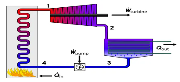
figure1 : Rankine cycle

• The Rankine cycle is an idealized thermodynamic cycle describing the process by which certain heat engines. Such steam turbines or reciprocating steam engines, allow mechanical work to be extracted from a fluid as it moves between a heat source and heat sink.
• Heat energy is supplied to the system via a boiler where the working fluid is converted to a high-pressure gaseous state (steam) to turn a turbine. After passing over the turbine, the fluid can condense back into a liquid state as waste heat energy is rejected before being returned to the boiler, completing the cycle.
• There are four processes in the Rankine cycle.

1. Process 1-2 :- It is isentropic expansion. The dry saturated vapor expands through a turbine, generating power. This decreases the temperature and passes of the vapor, and some condensation may occur.
2. Process 2-3 :- It is constant pressure heat rejection in the condenser. The wet vapor then enters a condenser, condensed at a constant pressure to become saturated liquid.
3. Process 3-4 :- It is isentropic compression. The working fluid is pumped from low to high pressure. As the fluid is a liquid at this stage. The pump requires little input energy.
4. Process 4-1 :- The boiler has constant pressure heat addition. The high-pressure liquid enters a boiler, where it is heated at constant pressure by an external heat source to became a dry saturated.

NET WORK= Turbine work- Pump work

Back Work Ratio= pump work / Turbine work

PROGRAM CODE

clear all
close all
clc
%c%user inputs

fprintf("\n           Rankine cycle simulator   ");
fprintf("\n\n 1-2 is isentropic expansion in the turbine ");
fprintf("\n 2-3 is constant pressure heat rejection by the condenser");
fprintf("\n 3-4 is isentropic compression in the pump");
fprintf("\n 4-1 is constant pressure heat addition by the boiler\n");
p1=input("\n Enter the pressure at the turbine inlet (in bar):")
t1=input("\n enter the temperature at the turbine inlet (in degree celcius):");
p2=input("\n enter the pressure at the condenser(in bar):");

%c%calculation
p4=p1; %c%constant pressure heat addition
p3=p2; %c%constant pressure heat rejection
h1=XSteam('h_pT',p1,t1);
s1=XSteam('s_pT',p1,t1);
s2=s1; %C% isentropic expansion
t3=XSteam('Tsat_p',p3);
v3=XSteam('vL_p',p3);
s3=XSteam('sL_p',p3);
h3=XSteam('hL_p',p3);
t2=t3;
s4=s3; %c%isentropic compression
sf2=XSteam('sL_p',p2);
sg2=XSteam('sV_p',p2);
hf2=XSteam('hL_p',p2);
hg2=XSteam('hV_p',p2);
%c%  s2=sf2+x2(sfg2) 
%c% sfg2= sg2-sf2
%c% dryness fraction, x= (s2-sf2)/(sg2-sf2)
x2= (s2-sf2)/(sg2-sf2);
h2= hf2+(x2*(hg2-hf2));
h4=XSteam('h_ps',p4,s4);
cp4=XSteam('Cp_ps',p4,s4);
cv4=XSteam('Cv_ps',p4,s4);
gamma4= cp4/cv4;
%c% to calculate t4
%c% p4^(gamma-1)*t4^gamma=p3^(gamma-1)*t3^gamma
t4=(t3*((p4/p3)^((gamma4-1)/gamma4)));

%c% calculation 
 %c% workdone by turbine
 Wt= h1-h2;
 
 %c% workdone by pump
 Wp= h4-h3;
 
 %c% net workdone 
 W_net= Wt-Wp;
 
 %c% heat supplied 
 q_s=h1-h4;
 
 %c% heat rejected 
 q_r= h2-h3;
 
 % thermal efficiency in percentage 
 eff= (W_net/q_s)*100;
 
 % specific steam conception
 SSC= 3600/W_net;
 
 % back work ratio
  BWR=Wp/Wt;
 
 
 %c% plot Temperature vs Entropy
 figure(1)
 %c% plot the liquid and vapour saturation curves
 t=linspace(0,450,450);
 for i= 1:length(t)
   s_L(i)=XSteam('sL_T',t(i));
   s_V(i)=XSteam('sV_T',t(i));
 endfor
plot(s_L,t,'color','g')
hold on 
%c% plot 1-2 state
plot([s1,s2],[t1,t2],'color','b')

plot(s_V,t,'color','g')

%c% plot 2-3
plot([s2,s3],[t2,t3],'color','b')

%c% plot 3-4
plot([s3,s4],[t3,t4],'color','b')

%c% plot 4-1
tL=XSteam('Tsat_p',p1); % saturated temperature at p1
sL=XSteam('sL_T',tL);   % entropy at saturated temperature tL
plot([s4,sL],[t4,tL],'color','b') 

tV=tL; % same temperature 
sV=XSteam('sV_T',tV); % entropy at saturated temperature tV
plot([sL,sV],[tL,tV],'color','b')

plot([sV,s1],[tV,t1],'color','b')

grid on
% indicates state with number
text(s1,t1,'   1')
text(s2,t2,'   2')
text(s3,t3,'   3')
text(s4,t4,'     4')
title('Temperature vs Entropy')
xlabel('Entropy')
ylabel('Temperature')
legend('saturation curve','rankine cycle')

%c% plot Enthalpy vs Entropy
figure(2)
%c% plot liquid and vapour saturation curve
t=linspace(0,450,450);
for i=1:length(t)
h_L(i)=XSteam('hL_T',t(i));
h_V(i)=XSteam('hV_T',t(i));
endfor
plot(s_L,h_L,'color','g')
hold on
%c% plot 1-2
plot([s1,s2],[h1,h2],'color','b')

plot(s_V,h_V,'color','g')
 
%c% plot 2-3
s2_3=linspace(s3,s2,100);
for i=1:length(s2_3)
  h2_3(i)=XSteam('h_ps',p2,s2_3(i));
endfor
plot(s2_3,h2_3,'color','b')

%c% plot 3-4
plot([s3,s4],[h3,h4],'color','b') 

%c% plot 4-1
s4_1=linspace(s4,s1,100);
for i=1: length(s4_1)
  h4_1(i)=XSteam('h_ps',p1,s4_1(i));
endfor
plot(s4_1,h4_1,'color','b')
grid on

%c% indicates state with number
text(s1,h1,'   1')
text(s2,h2,'   2')
text(s3,h3,'   3')
text(s4,h4,'     4')
title('Enthalpy vs Entropy')
xlabel('Entropy')
ylabel('Enthalpy')
legend('saturation curve','rankine cycle')

% result output
fprintf('\n \n%37s','RESULT')
fprintf('\n \n%s %50s','At state point 1','At state point 2');
fprintf('\n %s %2.2f%s %39s %2.2f%s','p1 is :',p1,'bars','p2 is :',p2,'bars')
fprintf('\n %s %3.2f%s %28s %3.2f%s','t1 is :',t1,'degree celcius','t2 is :',t2,'degree celcius')
fprintf('\n %s %4.2f%s %36s %4.2f%s','h1 is :',h1,'kJ/kg','h2 is :',h2,'kJ/kg')
fprintf('\n %s %1.4f%s %36s %1.4f%s','s1 is :',s1,'kJ/kgK','s2 is :',s2,'kJ/kgK')

fprintf('\n \n%s %50s','At state point 3','At state point 4');
fprintf('\n %s %2.2f%s %40s %2.2f%s','p3 is :',p3,'bars','p4 is :',p4,'bars')
fprintf('\n %s %3.2f%s %29s %3.2f%s','t3 is :',t3,'degree celcius','t4 is :',t4,'degree celcius')
fprintf('\n %s %4.2f%s %37s %4.2f%s','h3 is :',h3,'kJ/kg','h2 is :',h4,'kJ/kg')
fprintf('\n %s %1.4f%s %36s %1.4f%s','s3 is :',s3,'kJ/kgK','s4 is :',s4,'kJ/kgK')

fprintf('\n \n%36s %4.1f%s','Wt is :',Wt,'kJ/kg')
fprintf('\n %35s %1.4f%s','Wp is :',Wp,'kJ/kg')
fprintf('\n %35s %4.2f%s','W_net is :',W_net,'kJ/kg')
fprintf('\n %35s %2.2f%s','efficiency is :',eff,'%')
fprintf('\n %35s %4.2f%s','SSC is :',SSC,'kJ/kwh')
fprintf('\n %35s %1.4f','Back work ratio is :',BWR)

RESULT

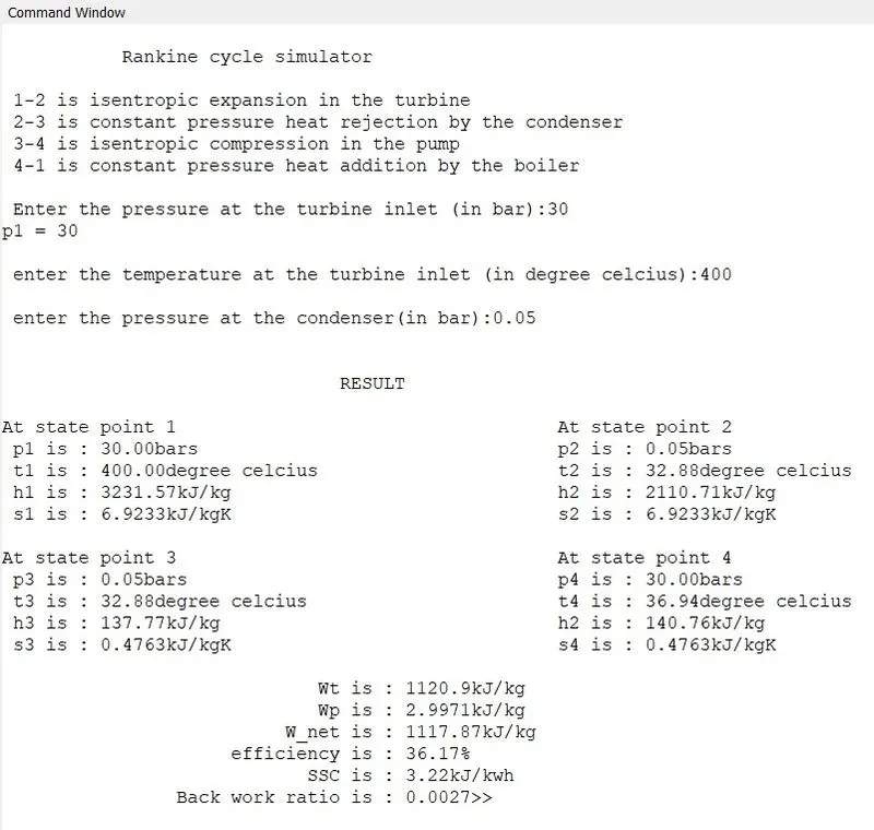
figure 2: result

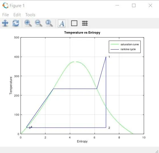
figure 3: Temperature vs Entropy

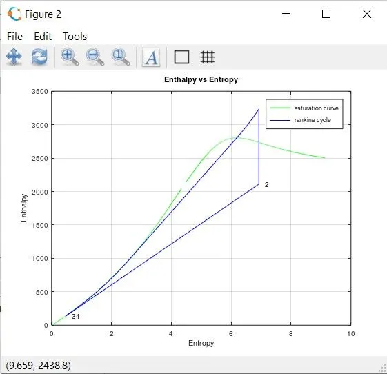
figure 4 : Enthalpy vs Entropy

EXPLANATION

• Using fprintf command to print the processes involved in the Rankine cycle.
• Using input command to display the prompt at command to get input values.
• Read the XSteam.m code carefully and use it to obtain the values of the thermodynamic properties at different states.
• We need at least 2 independent state properties to define other state properties using XSteam function.
• During phase changes, the temperature remains constant.
• Calculated the efficiency, network, back work ratio.
• During temperature vs entropy plotting,
• saturation curves plotted by finding saturated entropy property with respect to temperature range.
• Graph lines of straight lines are plotted directly, those are processed 1-2,2-3 and 3-4.
• Graph line of process 4-1 splitting into three parts. The first one is in between point 4 and saturated entropy point at pressure p1, the second one is in between saturated vapor entropy at pressure p1 and saturated liquid entropy at the same pressure, and the third one is in between saturated vapor entropy at pressure p1 and point 1.
• Each point is named in the graph using the text command.
• During enthalpy vs entropy plotting,
• Saturation curves plotted by finding saturated enthalpy property with respect to temperature range.
• Graph lines of straight lines are plotted directly, those are processes 1-2 and 3-4.
• Graph lines of processes 4-1 and 2-3 are plotted by finding intermediate values of enthalpy.
• Each point is named in the graph using the text command.
• The result outputs are displayed by using the fprintf command, those are thermodynamic properties of each state, net work, back work ratio etc.

CONCLUSION

• It is the simple Rankine cycle.
• H-S and T-S graphs are plotted.
• Efficiency and back work ratio are calculated