Week 3 - Solving second order ODEs

AIM

Write a program in matlab that will simulate pendulum motion.

To write a program that solves the following ODE. This ODE represents the equation of motion of simple pendulum with damping.

Governing equation

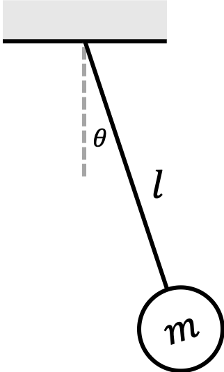
In Engineering, ODE is used to describe the transient behaviour of a system. A simple example is a pendulum. The way the pendulum moves depends on the newtons second law. When this law is written down, we get a second order ordinary differential equation that describes the position of the ball with respect to time.

In the above equation,

g = Gravity in m/

L = Length of the pendulum in m.

m = Mass of the ball in kg.

b = Dambing coefficient

FUNCTION PROGRAM

function[dtheta_dt]=ode_func(t,theta,b,g,l,m)
theta1=theta(1)
theta2=theta(2)
dtheta1_dt=theta2;
dtheta2_dt=-(b/m)*theta2-(g/l)*sin(theta1);
dtheta_dt=[dtheta1_dt;dtheta2_dt];
end

MAIN PROGRAM

clear all
close all
clc
% input data
b=0.05; % damping coefficient
g=9.81; % acceleration due to gravity
l=1; % length of pendulum
m=0.1; % mass of pendulum
% initial condition 
theta_0=[0;3]; % input of  angular displacement(rad) and angular velocity (rad/s)
% time points 
t_span=linspace(0,20,500);
% solve ODE
[t,results]=ode45(@(t,theta)ode_func(t,theta,b,g,l,m),t_span,theta_0);
% ploting section
figure(1)
plot(t,results(:,1))
ylabel('Angular displacement')
xlabel('time')
figure(2)
plot(t,results(:,2))
ylabel('Angular velocity')
xlabel('time')
% to create pendulum animation
theta1=results(:,1);
ct=1;
for i=1:length(theta1)
    THETA= theta1(i);
    %initial coordinate
    x0=0;
    y0=0;
    %final coordinate
    x1=l*cos((pi/2)-THETA);
    y1=-l*sin((pi/2)-THETA);
    figure(3)    
    plot([x0 x1],[y0 y1],'color','b','LineWidth',3) % to create string of pendulum
    line(x0,y0,'Marker','o','markersize',6,'MarkerFaceColor','g') % to create fixed point 
    line(x1,y1,'Marker','o','MarkerSize',20,'MarkerFaceColor','r') % to create bob
    line([-1 1],[0 0],'color','g') % to create pendulum holder
    axis([-1.25 1.25 -1.25 0.25]) % to define axis length
    title('Pendulum Animation')
    xlabel('xaxis')
    ylabel('yaxis')
    pause(0.03)
    M(ct)=getframe(gcf);
    ct=ct+1;
end
% to create video
movie(M)
videofile=VideoWriter('pendulum_animation.avi') % avoiding uncompressed due to large size
open(videofile)
writeVideo(videofile,M)
close(videofile)

RESULT

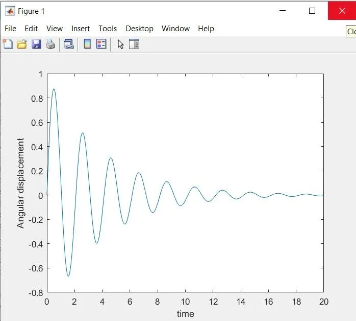
• Angular displacement vs Time

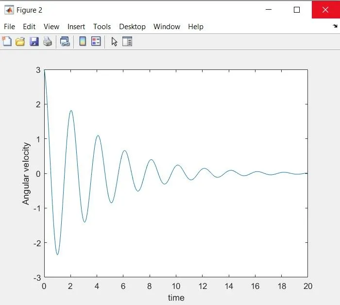
• Angular velocity vs Time
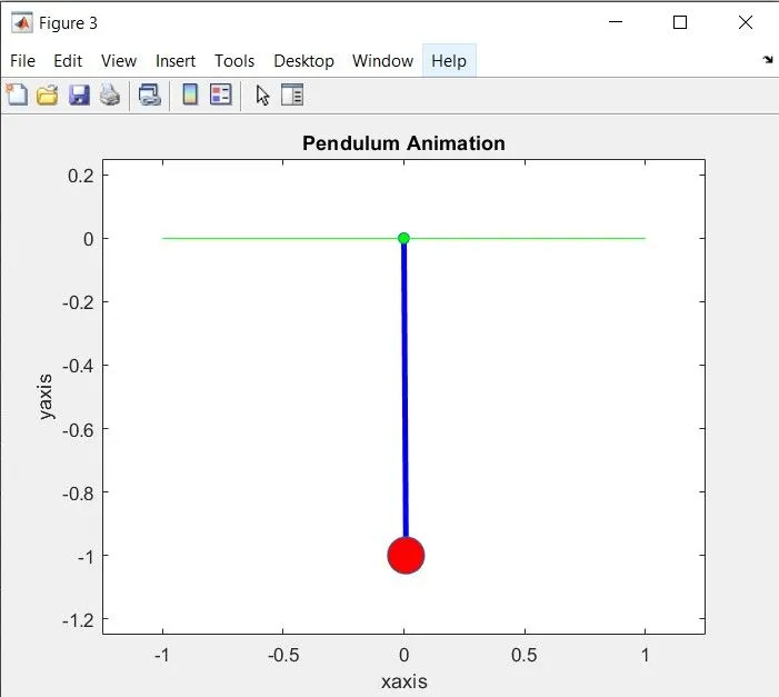
• Animation of pendulum

google drive link is given below

pendulum animation google drive link

EXPLANATION

Given data:-

g = 9.81 m/

l = 1m

m = 1kg

b = 0.05

time interval = 0 – 20 seconds

angular velocity at (t = 0) = 3 rad/s

• Input the given data of g, l , m ,b.
• Input the initial condition that is displacement and velocity at time 0 sec.
• Input the time points , that is 0 to 20 seconds asper the given data using linspace command.
• For solving ODE , changing the second or der ODE to first order ODE , that is in the function definition of function ‘ode_func.m’ and using ode45 command integrate this system of differential equation in interval of t_span with initial conditions theta_0.
• The syntax of ode45 is [t,y]= 0de45(odefun,tspan,y0)

Where tspan = [t0 tf] , integrate the system of differential equations y’ =f(t,y) from t0 to tf with initial condition y0. Each row in the solution array y corresponds to a value returned in column vector t.

• Here the ode45 command is

[t,results] = ode45(@(t,theta)ode_func(t,theta,b,g,l,m),t_span,theta_0);

Here t and theta are the variable of ode45 . ode_func is the function containing statements which change the second order equation to first order. t_span and theta_0 are the input data of t and theta. Output of the ode45 is results, which is an array of first coloumn contain displacement change with respect to time and second column containing angular velocity change with respect to time.

• Angular displacement vs time graph is plotted using command plot(t,results(:,1)).
• Angular velocity vs time graph is plotted using command plot(t,results(:,2)).
• To create pendulum animation

1. Using angular displacement values with respect to time is used to make the pendulum animation.
2. Assign the values of displacement to another variables, that is

theta1=results(;,1);

1. Pendulum in which one end is fixed . So x0= 0 and y0 = 0 .
2. Other end calculated using the sin and cos function.

That is , x1 = l*cos((pi/2)-THETA);

y1 =l*sin((pi/2)-THETA);

Here (pi/2) is added inside the cos and sin function because there is a need of shift of axis of equilibrium to vertical.

There is a -ve sign to y value because of pendulum oscillate below the xaxis.

• Plotting section

3. To create string of pendulum using plot command with color of blue and linewidth of 3.
4. To create fixed point at x0 and y0 using line command with marker of circle of size 6 and face color green.
5. To create bob at x1 and y1 using line command with marker of circle of size 20 and facecolor red.
6. To create pendulum holder using line command with green color.
7. Each frame is stored in array of M using getframe command.
8. All these steps under plotting section repeated with number of elements in theta1.Because all these are in for loop.

• To create a video of pendulum animation using movie command and save as pendulum_animation.avi.

CONCLUSION

• Matlab can be used for solving the ode of any order. Output of the displacement and velocity getting reduced with respect to time because of the damping provided.
• That is showed in the animation, that is oscillation of pendulum reduced with respect to time.