Week 4.1 - Genetic Algorithm

AIM

Write a code in MATLAB to optimize the stalagmite function and find the global maxima of the function.

Stalagmite function given :-

f(x,y) = f(1,x) × f(2,x) ×f(1,y) ×f(2,y)

f(1,x) =`[sin⁡( 5.1 πx+0.5)]^6`

f(2,y) =`[sin⁡( 5.1 πy+0.5)]^6`

f(2,x) =`e^([-4 ln⁡(2) (x-0.0667)^2/0.64])`

f(2,y) =`e^([-4 ln⁡(2) (y-0.0667)^2/0.64])`

OPTIMIZATION

Optimization is a decision-making process, it helps to find the best results under a set of prioritized criteria or constraints. Optimization aims to find that point or set of points in the search space.

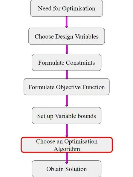
Figure 1. optimization flowchart

Here a stochastic method is used for optimization. The stochastic method is gaining popularity due to certain properties which deterministic algorithms do not possess. Stochastic models possess some inherent randomness, it is the probabilistic approach. Here genetic algorithm chooses as an optimization algorithm.

GENETIC ALGORITHM

A genetic algorithm is a search-based optimization technique based on genetics and natural selection principles. GA is categorized as global search heuristics. The evolution usually starts from a population of randomly generated individuals and happiness in generations. In each generation, the fitness of every individual in the population is evaluated, multiple individuals are selected from the current population based on their fitness, and modified to form a new population.

Working of GA :-

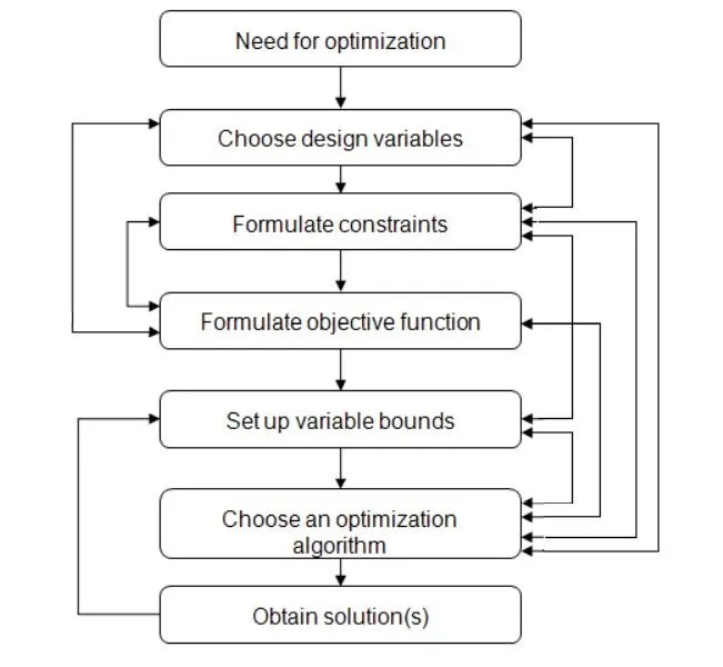
figure 2. Genetic algorithm flow chart

• Genetic algorithm optimization starts with population initialization.
• In the initialization, first we have to decide the population size. Higher the population size, we will get more combinations. Hence we get more accurate results. The population is the number of sample data points taken to perform the genetic algorithm operation.
• Selection process, in which the parents are selected from the sample data points, here roulette wheel rotated with fixed point and made so that the fitter individual has a high probability of becoming a parent.
• In the cross over process taking selected two parents and producing the children from them by interchanging the genes.
• Mutation is carried out to maintain the genetic diversity from one generation of a population of chromosomes to the next. In this process, the genes will be replaced by random integers.
• Replace the current population with the children to form the next generation.
• The algorithm stops when one of the stopping criteria is met.
• The algorithm takes modified steps for linear and integer constraints.
• The algorithm is further modified for nonlinear constraints.

STOPPING CRITERIA

• Max generations :- The algorithm stops when the number of generations reaches max generations.
• Max time :- The algorithm stops after running for an amount of time in seconds equal to max time.
• Fitness limit :- The algorithm stops when the value of the fitness function for the best point in the current population is less than or equal to the fitness limit.
• Max stall generations :- The algorithm stops when the average relative change in the fitness function value over Max stall generations is less than function tolerance.
• Max stall time :- The algorithm stops if there is no improvement in the objective function during an interval of time in seconds equal to max stall time.
• Function tolerance :- The algorithm runs until the average relative change in the fitness function value over max stall generations is less than function tolerance.

Syntax of genetic algorithm

• For unbounded

x= ga(fun, nvars)

finds a local unconstrained minimum, x to the objective function, fun. “nvars” is the dimension ( number of design variables ) of fun.

• For bounded

x= ga(fun, nvars, A,b, Aeq, beq, lb,ub)

defines a set of lower and upper bounds on the design variables x .So that a solution is found in the range lb ≤ x ≤ ub.

(set A= [ ] and b=[ ] if no linear inequalities exist.)

(set Aeq = [ ] and beq = [ ] if no linear equalities exist.)

• For bounded with modified population size.

x= ga(fun, nvars, A, b, Aeq, beq, lb, ub, nonlcon, intcon, options)

minimizes with the default optimization parameters replaced by values in options. Create options using “optimoptions”.

( set nonlcon= [ ] if non linear constraints exist.)

CODE FOR stalagmite FUNCTION

function[value]=stalagmite(v)
x=v(1);
y=v(2);
f1x=(sin(5.1*pi*x+0.5))^6;
f1y=(sin(5*pi*y+0.5))^6;
f2x=exp((-4*log(2)*(x-0.0667)^2)/0.64);
f2y=exp((-4*log(2)*(y-0.0667)^2)/0.64);
value=-f1x*f1y*f2x*f2y;
end

CODE FOR get_stalagmite FUNCTION

function[f]=get_stalagmite(x,y)
% creating a 2 dimension mesh 
[xx yy] = meshgrid(x,y);
% evaluating the stalagmite function
for i= 1:length(xx)
   for j= 1:length(yy)
    input_vector(1)=xx(i,j);
    input_vector(2)=yy(i,j);
    f(i,j)=stalagmite(input_vector);
   end
end

MAIN PROGRAM CODE

clear all
close all
clc
x=linspace(0,0.6,150); % input x values
y=linspace(0,0.6,150); % input y values 
num_cases=60;    
f=get_stalagmite(x,y); % to evaluate stalagmite function
% study 1 - statistical behaviour
tic
for i= 1:num_cases
    [inputs,fopt(i)]=ga(@stalagmite,2); % to optimise stalagmite function
    xopt(i)=inputs(1); % optimum x value 
    yopt(i)=inputs(2); % optimum y value 
end
study1_time=toc % time for first study
figure(1)
subplot(2,1,1)
hold on
surfc(x,y,-f)
shading interp
plot3(xopt,yopt,-fopt,'Marker','o','markersize',5,'markerfacecolor','r')
xlabel('x values')
ylabel('y values')
zlabel('f values')
title('unbounded inputs')
subplot(2,1,2)
plot(-fopt)
xlabel('iteration')
ylabel('function maximum')

% study 2- statistical behaviour with upper and lower bounds
tic
for i= 1:num_cases
    % to optimise stalagmite function
    [inputs,fopt(i)]=ga(@stalagmite,2,[],[],[],[],[0;0],[0.6;0.6]);
    xopt(i)=inputs(1); % optimum x value
    yopt(i)=inputs(2); % optimum y value
end
study2_time=toc
figure(2)
subplot(2,1,1)
hold on 
surfc(x,y,-f)
shading interp
plot3(xopt,yopt,-fopt,'Marker','o','markersize',5,'MarkerFaceColor','r')
xlabel('x values')
ylabel('y values')
zlabel('f values')
title('bounded inputs')
subplot(2,1,2)
plot(-fopt)
xlabel('iteration')
ylabel('function maximum')

% study 3 increasing GA population
options= optimoptions('ga')
options= optimoptions(options,'PopulationSize',170);
tic
for i=1:num_cases
    % to optimise stalagmite function
    [inputs,fopt(i)]=ga(@stalagmite,2,[],[],[],[],[0;0],[0.6;0.6],[],[],options);
    xopt(i)=inputs(1); % optimum x value 
    yopt(i)=inputs(2); % optimum y value
end
study3_time= toc
figure(3)
subplot(2,1,1)
hold on
surfc(x,y,-f)
shading interp
plot3(xopt,yopt,-fopt,'marker','o','MarkerSize',5,'MarkerFaceColor','r')
xlabel('x values')
ylabel('y values')
zlabel('f values')
title('bounded inputs with modified population size')
subplot(2,1,2)
plot(-fopt)
xlabel('iteration')
ylabel('function maximum')

RESULT

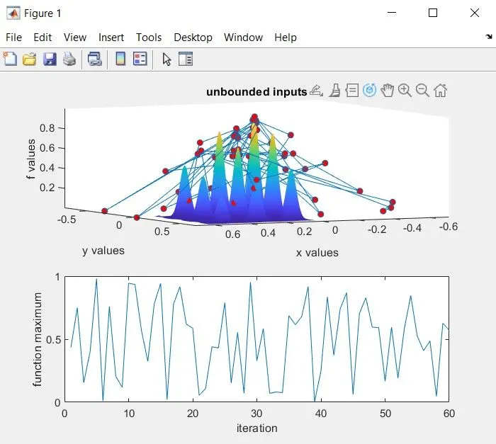
figure3. result of unbounded

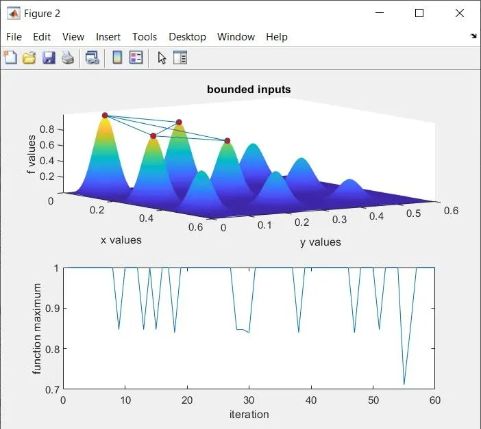
figure 4. result of bounded

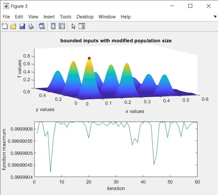
figure 5. result of bounded with modified population

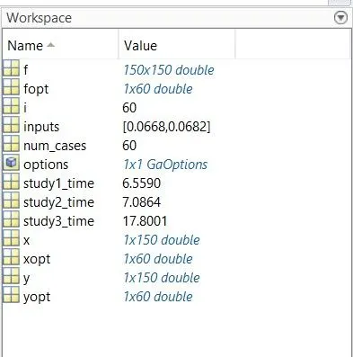
figure 6. workspace

EXPLANATION

• Initially changed the stalagmite function to get global maxima. That is the duality principle helps by allowing the same algorithm to be used for minimization and maximization with a minor change in the entire algorithm. Here the algorithm is for solving a minimization problem. It can be easily changed to a maximization problem by multiplying the objective function by -1 and vice versa.
• There are two functions is used one is an objective function “stalagmite” and the other is “get_stalagmite” which is used for evaluating the stalagmite function.
• There are three studies carried, the first one is statistical behavior. Here genetic algorithm is used to the optimum value of function through 60 iterations. Then surface plotting and 3d line plotting are carried. We can see that stalagmite surfaces with local maxima and global maxima. But maximum function value is varied all over the randomly. Because here optimization carried with no upper and lower bound. The graph of function maximum varies with iterations is shown in the figure. The negative sign in the plot and surf command is used to change the function values to positive values.
• The next study is a genetic algorithm with bounds. Accuracy increased with help of specified bounds. Again the function maximum varies small amount. We need to converge function maximum to a single point.
• Next study is bounded with modifying population, here along with bounds increasing the population size ( here is 170). Here function maximum optimized to a single point. We can see slight variations in “fopt” vs “ iteration” graph.

CONCLUSIONS

• GA is search-based optimization technique, so providing bounds improve accuracy.
• Using multiple iterations to increase the probability to get global maxima instead of local maxima.
• Increasing the population to increase the search space to get accurate results.

REFERENCE

• https://skill-lync.com/knowledgebase/genetic-algorithm-explained
• https://in.mathworks.com/help/gads/how-the-genetic-algorithm-works.html#f6243