Project 1 - Parsing NASA thermodynamic data
AIM
To parse a thermodynamics file by NASA.
Objective
- To extract the coefficients from the file for each species.
- To calculate the molecular weight of each species.
- Plot the specific heat , enthalpy & entropy graphs concerning their local temperature.
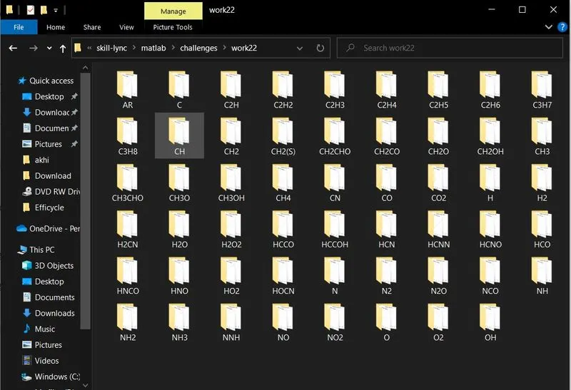
- Save the plots in respective folders of the species.
Click here for the thermodynamic file.
Description
The first 7 coefficient are high temperature coefficients and the second 7 coefficients are low temperature coefficients.
Theory
File parsing:-
File parsing refers to examining a file. Data can be extracted from the file and used to perform calculations. Also, data can be imported to the file. Here a thermodynamics file generated by NASA is parsed.
Specific heat capacity (cp)
Specific heat capacity is defined as the heat required to raise the temperature of given mass by a unit temperature. It is denoted as unit is J/k.
Enthalpy (H)
Enthalpy refers to the internal energy of a system which includes the temperature and pressure in an enclosed system. The change in heat is referred to as enthalpy of the system. It is denoted as H and the unit is J/mol.
Entropy (S)
Entropy is defined as a measure of randomness or disorder of a system. It is denoted as S. unit is J/k.
Formulas are given below.
CP/R = a1 + a2 T+ a3 T^2+ a4 T^3+ a5 T^4
H/RT= a1 + a2 T/2+ a3 T^2/3+ a4 T^3/4+ a5 T^4/5+ a6/T
S/R= a1 ln T+ a2 T+ a3 T^2/2+ a4 T^3/3+ a5 T^4/4+ a7
FUNCTION PROGRAM
function [CP,H,S]=calculator_properties(coeff,local_mid_temp,Temp)
a=coeff;
R = 8.3145;
 for i= 1: length(Temp)
     T= Temp(i);
    if T> local_mid_temp
        % using high temperature coefficients
         CP(i)= (a(1)+ a(2)*T +a(3)*T^2 +a(4)*T^3 +a(5)*T^4)*R;
         H(i)= (a(1)+ a(2)*T/2+ a(3)*(T^2)/3+ a(4)*(T^3)/4+ a(5)*(T^4)/5+ a(6)/T)*R*T;
         S(i)= (a(1)*log(T)+ a(2)*T+ a(3)*(T^2)/2+ a(4)*(T^3)/3+ a(5)*(T^4)/4+ a(7))*R;
    else
         % using low temperature coefficients
         CP(i)= (a(8)+ a(9)*T +a(10)*T^2 +a(11)*T^3 +a(12)*T^4)*R;
         H(i)= (a(8)+ a(9)*T/2+ a(10)*(T^2)/3+ a(11)*(T^3)/4+ a(12)*(T^4)/5+ a(13)/T)*R*T;
         S(i)= (a(8)*log(T)+ a(9)*T+ a(10)*(T^2)/2+ a(11)*(T^3)/3+ a(12)*(T^4)/4+ a(14))*R;
    end
 end
MAIN PROGRAM
clear all
close all
clc
f1= fopen('THERMO.dat','r')
fgetl(f1)
tline= fgetl(f1);
A= strsplit(tline,' ');
global_low_temp= str2num(A{2})
global_mid_temp= str2num(A{3})
global_high_temp= str2num(A{4})
% skipping next 3 lines
fgetl(f1)
fgetl(f1)
fgetl(f1)
for i= 1:53
    tline1=fgetl(f1);
    Z=strsplit(tline1,' ');
    n=length(Z);
    species_name= Z{1}
    local_low_temp= str2num(Z{n-3})
    local_mid_temp= str2num(Z{n-1})
    local_high_temp= str2num(Z{n-2})

    % first 7 coefficients are high temperature coefficients.
    tline2=fgetl(f1);
    B=findstr(tline2,'E');
    a1= str2num(tline2(1:B(1)+3));
    a2= str2num(tline2(B(1)+4:B(2)+3));
    a3= str2num(tline2(B(2)+4:B(3)+3));
    a4= str2num(tline2(B(3)+4:B(4)+3));
    a5= str2num(tline2(B(4)+4:B(5)+3));
    tline3= fgetl(f1);
    C=findstr(tline3,'E');
    a6= str2num(tline3(1:C(1)+3));
    a7= str2num(tline3(C(1)+4:C(2)+3));

    % second 7 coefficients are low tempterature coefficients
    a8= str2num(tline3(C(2)+4:C(3)+3));
    a9= str2num(tline3(C(3)+4:C(4)+3));
    a10= str2num(tline3(C(4)+4:C(5)+3));
    tline4= fgetl(f1);
    D= findstr(tline4,'E');
    a11= str2num(tline4(1:D(1)+3));
    a12= str2num(tline4(D(1)+4:D(2)+3));
    a13= str2num(tline4(D(2)+4:D(3)+3));
    a14= str2num(tline4(D(3)+4:D(4)+3));

    % for finding specific heat ,enthalpy and entropy.
    coeff= [a1,a2,a3,a4,a5,a6,a7,a8,a9,a10,a11,a12,a13,a14];
    Temp = local_low_temp :local_high_temp;
    [CP,H,S]= calculator_properties(coeff,local_mid_temp,Temp)
    specific_heat=CP;
    enthalpy= H;
    entropy=S;

    % creating a folder and changing current folder
   mkdir(['E:\skill-lync\matlab\challenges\work22\',species_name])
   cd(['E:\skill-lync\matlab\challenges\work22\',species_name])
   % plotting and saving section
   figure(1)
   plot(Temp,CP)
   grid on
   xlabel('temperature')
   ylabel('specific heat')
   text1=sprintf('temperature vs specific heat (%s)',species_name);
   title(text1)
   saveas(1,text1,'jpeg')

    figure(2)
  a= plot(Temp,H)
   grid on
   xlabel('temperature')
   ylabel('enthalpy')
   text2=sprintf('temperature vs enthalpy (%s)',species_name);
   title(text2)
   saveas(a,text2,'jpeg')

    figure(3)
   plot(Temp,S)
   grid on
   xlabel('temperature')
   ylabel('entropy')
   text3=sprintf('temperature vs entropy (%s)',species_name);
   title(text3)
   saveas(3,text3,'jpeg')


    % for finding molecular weight of species
   molecular_weight= 0;
   elements=['O','H','C','N','AR'];
   atomic_weight=[15.999,1.008,12.011,14.007,39.948];
   for l= 1:length(species_name)
      for j= 1: length(atomic_weight)
          if strcmp(species_name(l),elements(j))
           molecular_weight= molecular_weight+ atomic_weight(j);
           position =j;
          end
      end
      n=str2double(species_name(l));
      if n > 1
      molecular_weight= molecular_weight+ atomic_weight(position)*(n-1);
      end
   end
   sprintf('Molecular Weight of %s:%f u',species_name,molecular_weight)

   end
RESULT
- Screenshot of the window where all the folders are saved .
- Plots for O2
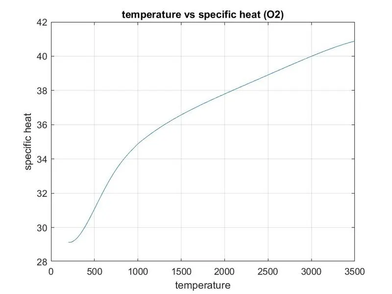
figure 1.1:- temperature vs specific heat
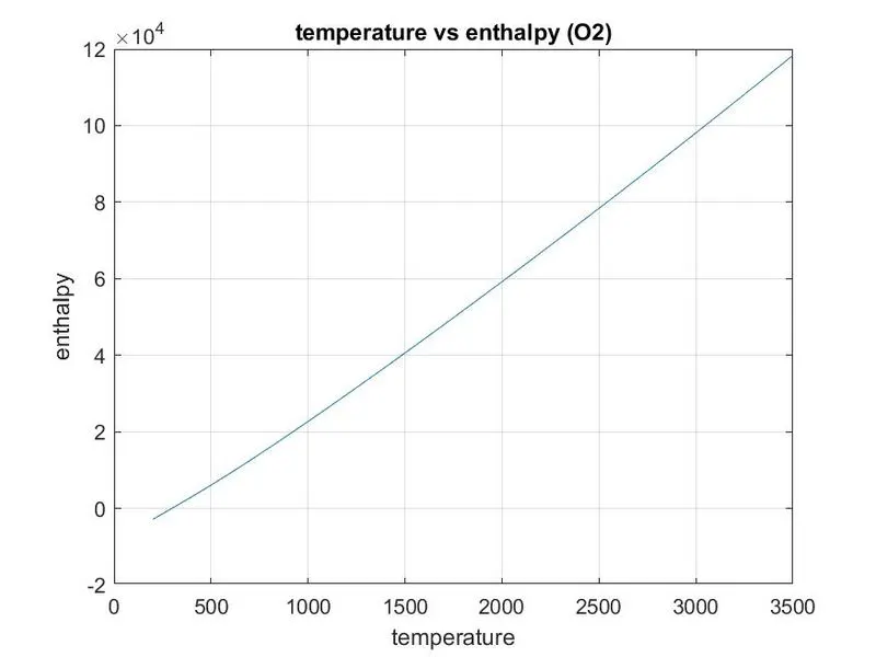
figure 1.2:- temperature vs enthalpy
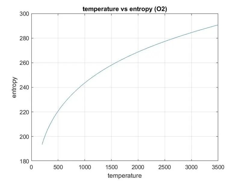
figure 1.3:- temperature vs entropy
- plots for N2
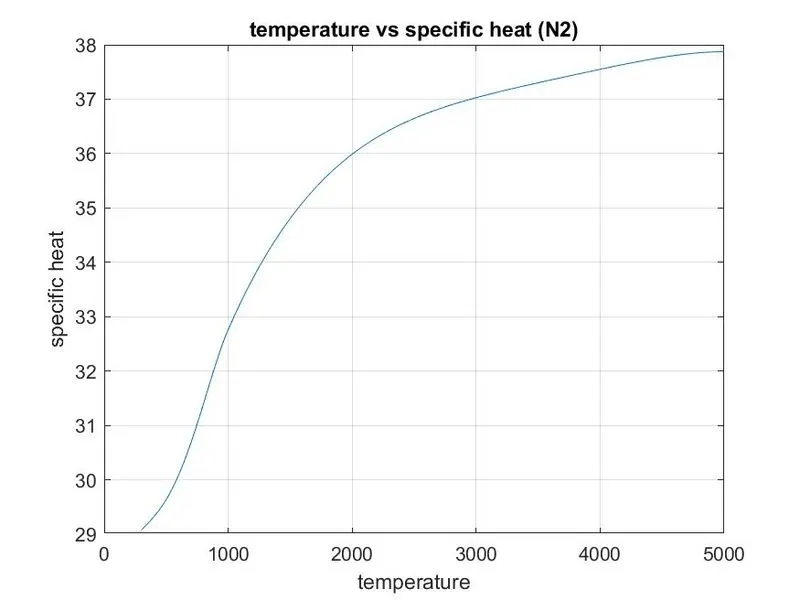
figure 2.1:- temperature vs specific heat
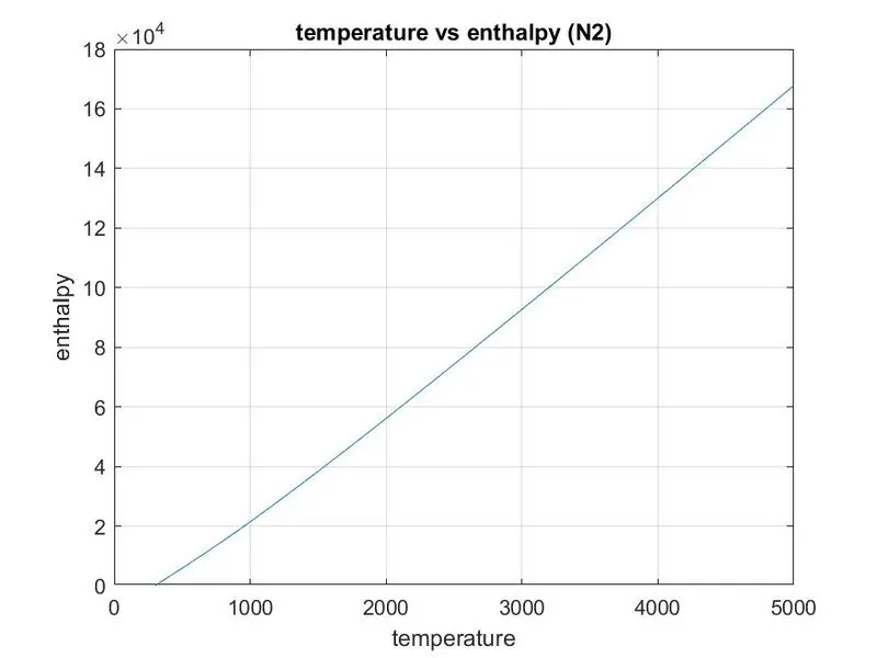
figure 2.2 :- temperature vs enthalpy
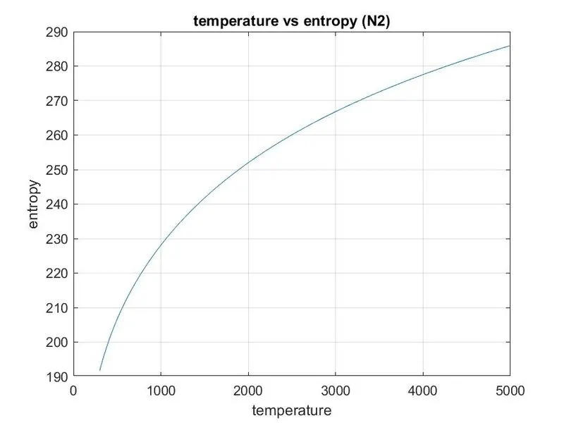
figure 2.3:- temperature vs entropy
- plots for CO2
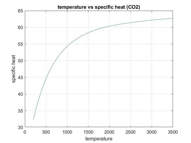
figure 3.1:- temperature vs specific heat
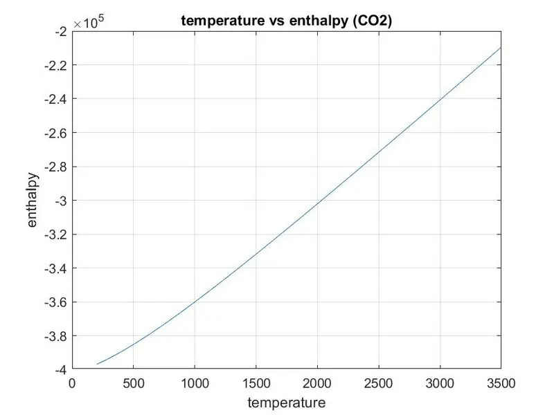
figure 3.2:- temperature vs enthalpy
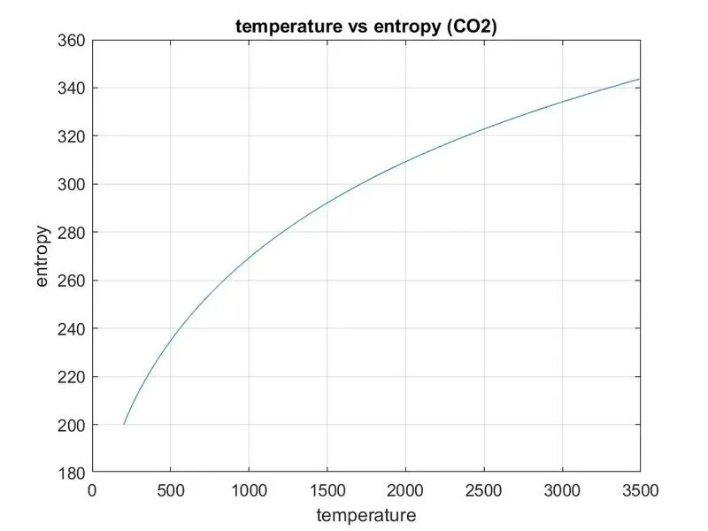
figure 3.3:- temperature vs entropy
Explanation
- File opened for reading using fopen command.
- Global temperatures are extracted using fgetl command, string splitting and converting string to number
- Here data line is saved to a variable, string splitting according to the space gap in the data line and each split data is a cell array. Each element is converted into a number and saved to the corresponding global temperature.
- 53 species are in the file. So for-loop is created with the number of loop is 53
- Data line is extracted using fgetl command and species name and temperature is extracted and saved to the corresponding variable.
- Here data line is saved to a variable, string splitting according to the space gap in the data line. The first element in the cell array is saved to species name and other corresponding elements in the cell array is converted into a number and saved to the corresponding local temperature.
- For extracting temperature coefficient extract the line using fgetl command. Each coefficient with exponent symbol, so find the locations of E in the data line and saved to another variable. Using this set of values call the data in the data line using array indices and convert it into numbers and saved it to coefficients, that is a1, a2,a3………a14.
- For calculating the specific heat, enthalpy and entropy. Create an array with all 14 coefficients and another array with local temperature. Create a function for calculating the CP,H &S and calling this function by passing coefficient array, temperature array and local mid temperature. The function returns 3 values that are saved to corresponding variables that are specific heat, enthalpy, entropy.
- Inside the function calculator_properties, there is a for-loop with the number of the loop is equal to the local temperature range. If-else command is used for matching temperature coefficients & temperature values in the equation.
- Create the folder with species name using the mkdir command.
- Change the current folder to species name folder for saving plots.
- CP,H & S plots are created and saved to the folder using save as command.
- For finding the molecular weight of species. Initially, molecular weight was set into zero. Create the elements array and atomic weight array. Comparing the species name and elements array, atomic weight added with the molecular weight if species name data element is equal to the element data element and position of atomic weight is saved else (n-1) times of atomic weight added with molecular weight. Where n is the number that in the species name data at a particular position.
- All the process under the loop is repeated for the next 52 species.
CONCLUSIONS
- Coefficients for each species extracted.
- Molecular weight of each species calculated.
- The graphs of CP, H & S with respect to their local temperature are plotted.
- The plots in respective folders of the species are saved.