Project 1
Aim:- Deals with the development of a forward energy-based fuel consumption model of a conventional vehicle.
Objectives:-
a. Tabulate the fuel economy numbers (kmpl) for UDDS and HWFET cycle. This forms the baseline numbers for comparing with the future hybrid version.
b. Plot the time trace for engine, transmission input, transmission output and wheel speed on one plot.
c. Plot engine torque, engine power, fuel rate and fuel consumption using subplots.
d. Plot accelerator and brake pedal, gear command, vehicle desired and actual speed, vehicle distance using subplots.
e. Plot the engine operating points on the engine fuel map.
f. Write down appropriate brief comments on each of these plots, describing the vehicle behavior throughout the drive cycle.
g. Generate the plots for both drive cycles
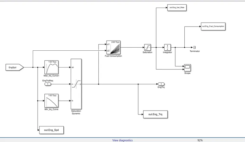
Complete the Engine block :-
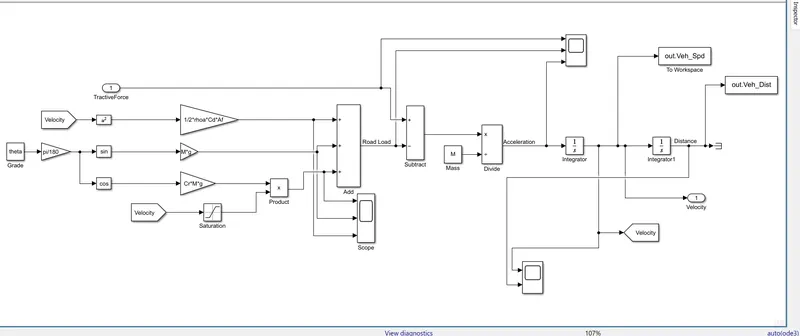
Complete the Vehicle Dynamic block :-
Modification in Matlab code for generate required plots:-
%%%%%%%%%%%%%%%%%%%%%%%%%%%%%%%%%%%%%%%%%%%%%%%%%%%%%%%%%%%%%%%%%%%%%
%% Skill-Lync -> Hybrid Drives Development
% Project 1 - Conventional Vehicle Model
% By - Ullekh Gambhira

% Description:
% The following file is to used with the Initialization file and Simulink
% results for post-processing of the data.
% The file is incomplete, has some examples of how the data is imported
% into a readable format, data analysis and plotting examples.
% Based on the project task, use commands in a similar format as given
% below, to analyse the data and generate required plots.
% You can change variable names if desired

%% Post-Processing File
%  File for post-processing the Conventional vehicle simulation model data

%% Renaming variables
Time = out.tout;
Acc_Pdl = out.Acc_Pdl;          % Accelerator pedal [%]
Brk_Pdl = out.Brk_Pdl;          % Brake pedal [%]
Gear_Cmd = out.Gear_Cmd;        % Transmission gear
Trans_In_Spd = out.Trans_In_Spd*30/pi;  % Transmission input speed [rpm]
Trans_Out_Spd = out.Trans_Out_Spd*30/pi;% Transmission output speed [rpm]
Eng_Trq = out.Eng_Trq;          % Engine brake torque [Nm]
Eng_Spd = out.Eng_Spd*30/pi;    % Engine speed [rpm]
Eng_Fuel_Consump = out.Eng_Fuel_Consumption;    % Engine fuel consumption [g]
Veh_Dist = out.Veh_Dist/1000;   % Distance traveled by vehicle [km]
Veh_Spd = out.Veh_Spd*18/5;     % Vehicle speed [kmph]
Eng_fuel_Rate= out.Eng_fuel_Rate; % Engine fuel rate

%% Data Analysis
Eng_Pwr = Eng_Spd*pi/30.*Eng_Trq/1000;   % Engine brake power [kW]
rho_petrol = 0.7197;                    % Density of petrol [kg/L]
kmpl = Veh_Dist(end)/(Eng_Fuel_Consump(end)/1000/rho_petrol);    % Fuel economy [kmpl]


%% Plotting vehicle characteristics time trace
figure()
subplot(3,1,1)
hold on
grid on
plot(Time, Acc_Pdl, 'linewidth', 1, 'Color', 'black');
plot(Time, Brk_Pdl, 'linewidth', 1, 'Color', 'red');
ylabel('Pedal [%]')
xlim([0, Time(end)]);
legend('Accel','Brake');
subplot(3,1,2)
hold on
grid on
plot(Time, Trans_In_Spd, 'linewidth', 1, 'Color', 'black');
plot(Time, Trans_Out_Spd, 'linewidth', 1, 'Color', 'red');
ylabel('Speed [rpm]')
xlim([0, Time(end)]);
ylim([0, 6000]);
legend('Trans Input','Trans Output');
subplot(3,1,3)
hold on
grid on
plot(Time, Gear_Cmd, 'linewidth', 1, 'Color', 'black');
xlim([0, Time(end)]);
xlabel('Time [s]');
ylabel('Gear');


%% Plotting engine operating points on engine fuel map
figure('Name','Engine Operating Points');
hold on
grid on
title('Engine Operating Points','fontsize',12);
p1=plot(Eng_map_spd*30/pi,Eng_max_trq,'linewidth',2,'color','r');
p2=line([Eng_map_spd(end)*30/pi Eng_map_spd(end)*30/pi],[0 Eng_max_trq(end)]);
set(p2,'linewidth',1,'linestyle','--','color','k');
p3=line([Eng_map_spd(1)*30/pi Eng_map_spd(1)*30/pi],[0 Eng_max_trq(1)]);
set(p3,'linewidth',1,'linestyle','--','color','k');
[c,h] = contour(Eng_map_spd'*30/pi,Eng_map_trq,Eng_fuel_map');
clabel(c,h);
xlabel('Engine Speed [rpm]');
ylabel('Engine Torque [Nm]');
title('Engine Fuel Consumption Map [g/s]');
%p4 = plot(Eng_Spd,Eng_Trq,'.','color','k');
legend([p1 p3],{'Max Curve','Operating Points'});
axis([Eng_map_spd(1)*30/pi Eng_map_spd(end)*30/pi 0 Eng_map_trq(end)]);

figure(3)
subplot(3,1,1)
hold on
grid on
plot(Time, Eng_Trq, 'linewidth', 1, 'Color', 'black');
xlim([0, Time(end)]);
xlabel('Time [s]');
ylabel('Engine Torque');

subplot(3,1,2)
plot(Time, Eng_Pwr, 'linewidth', 1, 'Color', 'black');
xlim([0, Time(end)]);
xlabel('Time [s]');
ylabel('Engine Power');

subplot(3,1,3)
hold on
grid on
plot(Time, Eng_fuel_Rate, 'linewidth', 1, 'Color', 'black');
plot(Time, Eng_Fuel_Consump, 'linewidth', 1, 'Color', 'red');
ylabel('Engine fuel [%]')
xlim([0, Time(end)]);
legend('Fuel rate','Fuel consumption','Location','best');

figure(4)
subplot(2,2,1)
hold on
grid on
plot(Time, Acc_Pdl, 'linewidth', 1, 'Color', 'black');
plot(Time, Brk_Pdl, 'linewidth', 1, 'Color', 'red');
ylabel('Pedal [%]')
xlim([0, Time(end)]);
legend('Accel','Brake');

subplot(2,2,2)
hold on
grid on
plot(Time, Gear_Cmd, 'linewidth', 1, 'Color', 'black');
xlim([0, Time(end)]);
xlabel('Time [s]');
ylabel('Gear');

subplot(2,2,3)
hold on
grid on
plot(Time, Veh_Spd, 'linewidth', 1, 'Color', 'black');
xlim([0, Time(end)]);
xlabel('Time [s]');
ylabel('Vehicle speed');


subplot(2,2,4)
hold on
grid on
plot(Time, Veh_Dist, 'linewidth', 1, 'Color', 'black');
xlim([0, Time(end)]);
xlabel('Time [s]');
ylabel('Vehicle distance');
Blocks used :-
1.goto and from block -goto and from block
2.1-D lookup table -The 1-D, 2-D, and n-D Lookup Table blocks evaluate a sampled representation of a function in N variables
3.Saturation Dynamic -Limit input signal to dynamic upper and lower saturation values
4.To workspace -Log data to workspace from Simulink model
5.2-D lookup table -The 1-D, 2-D, and n-D Lookup Table blocks evaluate a sampled representation of a function in N variables
6.Saturation -Limit input signal to the upper and lower saturation values
7.Integrator -The Integrator block outputs the value of the integral of its input signal with respect to time.
8.Terminator -The Terminator block can be used to cap blocks whose output ports are not connected to other blocks.
9.Scope -Display signals generated during simulation
10.Constant -the Constant block outputs a signal whose data type and complexity are the same as those of the Constant value parameter.
11.Gain -A gain schedule converts the scheduling variables that describe the current operating condition into appropriate controller gains.
12.Square -Square the give values.
13.Sin - sin trigonometric function.
14.Cos - cos trigonometric function.
15.Product -The Product block performs multiplication or division of its inputs.
16.Add - This block performs the addition function.
17.Subtract -This block performs the subtract function.
18.Divide -This block performs the divide function.
Explanation:-
From above simulink blocks we create the Engine block and and Vehicle dynamics blocks for the conventional vehicle model.
and complete the conventional vehicle model.
after this we plot the required graph for the time trace for engine, transmission input, transmission output and wheel speed on one plot.Plot engine torque, engine power, fuel rate and fuel consumption using subplots. Plot accelerator and brake pedal, gear command, vehicle desired and actual speed, vehicle distance using subplots.Plot the engine operating points on the engine fuel map.and we Generate the plots for both drive cycles UDDS and HWFET.
FOR UDDS DRIVE CYCLE:-
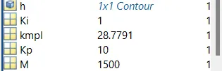
a) The fuel economy numbers (kmpl) for UDDS- 28.7791
b) Plot the time trace for engine, transmission input, transmission output and wheel speed on one plot.
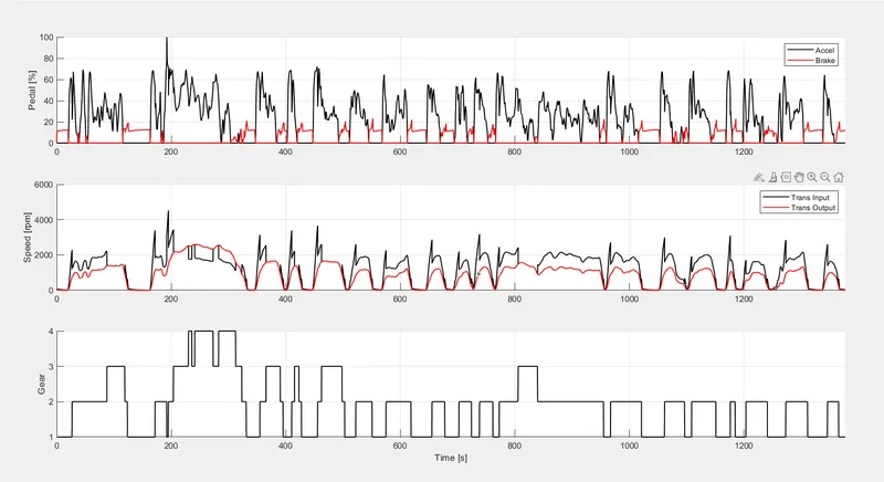
As we can see from above plot , when we give the power to the vehicle the speed increase and transmission power also increase and when we press the accelerator padel the speed will increase.in this cycle the fluctuating in speed and fuel consumption is very high.
c) Plot engine torque, engine power, fuel rate and fuel consumption using subplots.
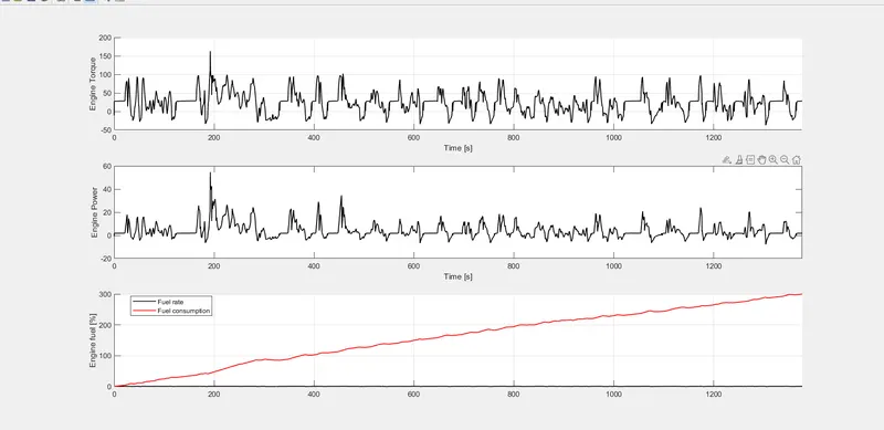
as we can see that when the torque is increase the engine power is also increase and because the torque increase the fuel consumption is also increase as well as fuel rate.in this cycle the fuel rate is high.
d) Plot accelerator and brake pedal, gear command, vehicle desired and actual speed, vehicle distance using subplots.
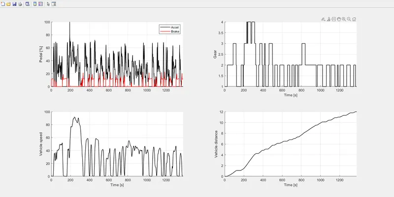
In the vehicle the accelerator padel is used for increase the speed of vehicle and brake padel is used for stop the vehicle and when accelerator padel is pressed the the vehicle speed as well as torque and power is also increase. in udds the use of accelerator and brake padel is more as compared to hwfet so for this cycle the fuel consumption is very high.
e) Plot the engine operating points on the engine fuel map.
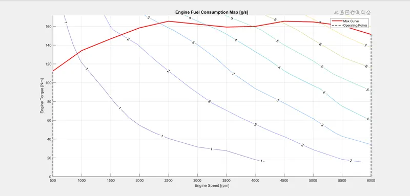
on the different operating conditions the fuel consumption is high and depends upon the raod load and torque range of the vehicle and various loads. in udds the map is show the more fuel consumption.
FOR HWFET DRIVE CYCLE:-
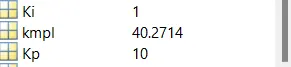
a) The fuel economy numbers (kmpl) for HWFET- 40.271
b) Plot the time trace for engine, transmission input, transmission output and wheel speed on one plot.
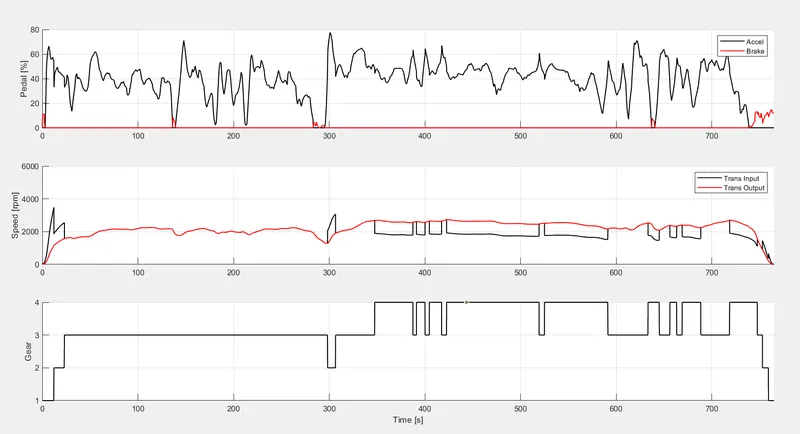
As we can see from above plot , when we give the power to the vehicle the speed increase and transmission power also increase and when we press the accelerator padel the speed will increase. in this cycle the vehicle is run constantly on the road so the fluctuation is less as compared to udds.
c) Plot engine torque, engine power, fuel rate and fuel consumption using subplots.
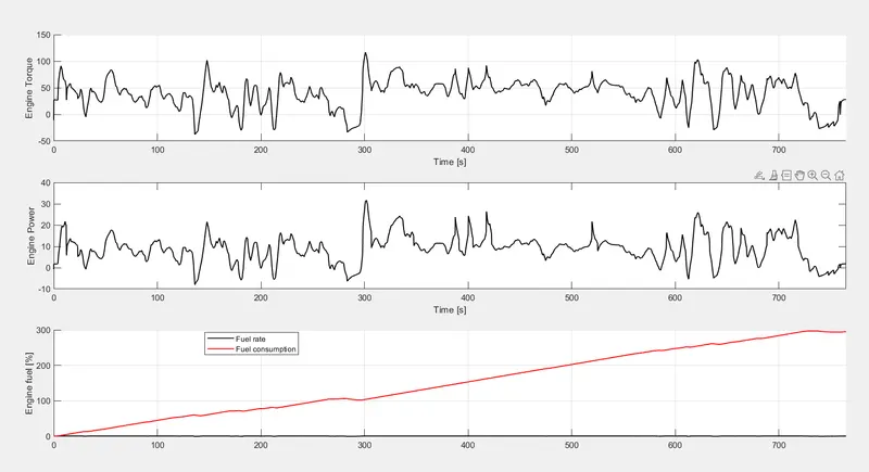
as we can see that when the torque is increase the engine power is also increase and because the torque increase the fuel consumption is also increase as well as fuel rate.in this cycle the fuel rate is in economy because the fuel consumption is uniform .
d) Plot accelerator and brake pedal, gear command, vehicle desired and actual speed, vehicle distance using subplots.
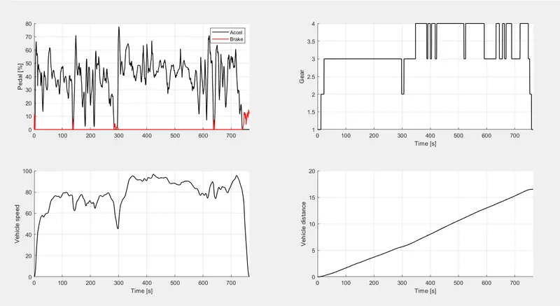
In the vehicle the accelerator padel is used for increase the speed of vehicle and brake padel is used for stop the vehicle and when accelerator padel is pressed the the vehicle speed as well as torque and power is also increase. In the HWFET the use of brake padel and accelerator padel is use very less because the vehicel is made to rum in highway roads.
e) Plot the engine operating points on the engine fuel map.
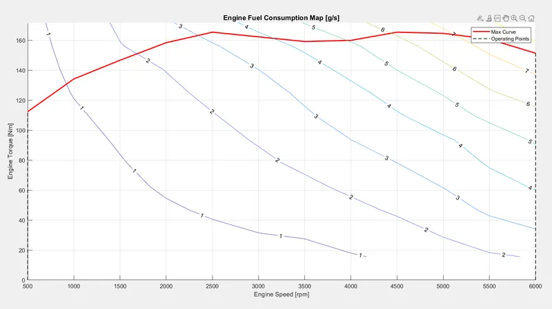
on the different operating conditions the fuel consumption is high and depends upon the raod load and torque range of the vehicle and various loads. in hwfet the engine speed is constant at maximum time and due to this the fuel consumption is economical.
Conclusion:-
Here we understand the conventional vehicle model and their different parameters and understand the working of sumulink models and different blocks. In this model we understand the modeling process and analyzing process and learn how to write the script for the different purposes.