Week 3 - Solving second order ODEs

Aim:- Write a program in Matlab that will simulate the pendulum motion by solving the second order ODE and create animation of it.

Simple pendulum:- A simple pendulum can be described as a device where its point mass is attached to a light inextensible string and suspended from a fixed support. The vertical line passing through the fixed support is the mean position of a simple pendulum. The vertical distance between the point of suspension and the centre of mass of the suspended body (when it is in mean position) is called the length of the simple pendulum denoted by L. This form of the pendulum is based on the resonant system having a single resonant frequency.

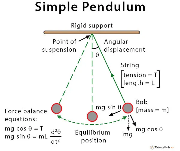
Simple harmonic motion:-Simple Harmonic Motion or SHM is defined as a motion in which the restoring force is directly proportional to the displacement of the body from its mean position. The direction of this restoring force is always towards the mean position.

Governing equations:-

*ODE representing equation of motion of a simple pendulum with damping -

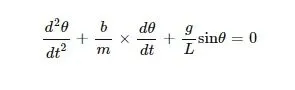
Where -

g = gravity (m/s^2)

L = length of pendulum (m)

m = mass of the ball (kg)

b = damping coefficient

Objective:-

1. To study the transient behavior of the pendulum system.

2. Animate the motion of simple pendulum.

Input values:-

g = 9.81 m/s^2

L = 1 metre

m = 1 kg

b = 0.05

time = 0-20 sec (for simulation)

angular displacement = 0

angular velocity = 3 rad/sec

MATLAB code:-

1.Code function of ode45 for main program-

function  [dtheta_dt] = ode_func(t,theta,b,g,l,m)
theta1 = theta(1);
theta2 = theta(2);
dtheta1_dt = theta2;
dtheta2_dt = -(b/m)*theta2-(g/l)*sin(theta1);
dtheta_dt = [dtheta1_dt;dtheta2_dt];
end

2.Main program-

% Program to solve 2nd order ODE 
clear all 
close all
clc

% Inputs
b  = 0.05;                    % damping coefficient 
g = 9.81;                     % gravity in m/s^2
l = 1;                        % length of the pendulum in metre
m = 1;                        % mass of the ball in kg

% Initial condition 
theta_0 = [0; 3];             % Defining angular displacement and angular velocity in array

% Time points 
t_span = linspace(0,20,250);  % Defining time for oscillation from 0 to 20sec

% Solve ODE
[t,results] = ode45(@(t,theta) ode_func(t,theta,b,g,l,m),t_span,theta_0);

figure(1)
plot(t,results(:,1))
hold on 
plot(t,results(:,2))
xlabel('time')
ylabel('plots')
legend('displacement','angular velocity')
grid on 
hold off

displacement = results(:,1);
velocity = results(:,2);

% Fixed coordinate 
x0 = 1;
y0 = 1;
ct = 1;

for i = 1:length(displacement)

    % Coordinates
    x1 = 1-l*sin(displacement(i));
    y1 = 1-l*cos(displacement(i));

    figure(2)
    %plot fixed link 
    plot([0 2],[1 1],'LineWidth',6,'color','y')
    hold on 
    plot([1 x1],[1 y1],[x1 x1],[y1 y1],'-o','markersize',25,'markerfacecolor','b','linewidth',4)
    plot(x0,y0,'-o','markersize',4,'markerfacecolor','g')
    
    % Axis setting 
    axis([0 2 -0.5 2])

    M(ct)= getframe(gcf);          % capture currant figure using getframe command 
    ct = ct+1;                     % loop counter 
    hold off 
   
end 
movie(M)                           % stiching all the frame in the M array to create animation 
videofile=VideoWriter('simple_pendulum.avi','uncompressed AVI');
open(videofile)
writeVideo(videofile,M)
close(videofile)

Code explations:-

*clera all- To clear all variables from current workplace.

*close all- close all figures whose handles are visible.

*clc - clc clears all the text from the command window.

*linspace()- This function will generate a vector of values linearly spaced between two endpoints.

*ode45- It's the MATLAB’s standard solver for ordinary differential equations (ODEs).

*ode_func- it is the function code which is separately create to solve 2nd oder ode.

*plot()- creates a 2-D line plot .

*hold on -it retains the current plot and certain axes properties so that subsequent graphing commands add to the existing graph.

*xlabel()- It labels the x-axis of the current plot.

*ylabel()- It labels the y-axis of the current plot.

*legend()-legend creates a legend with descriptive labels for each plotted data series.

*grid on- It displays grid lines.

*hold off- it sets the hold state to off so that new plots added to the axes clear existing plots and reset all axes properties.

*getframe()-it is used in a for loop to assemble an array of movie frames for playback using movie.

*Videowriter()-to create a video file from an array.

Results:-

Outputs-

1.Graph

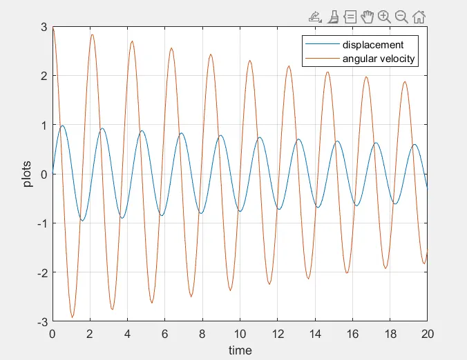
The displacement (blue color) and angular velocity (red color) is decreasing with increasing in time this is due to damper ,i.e damping coefficient which absorbs the variations to make the body in equillibrium position.

2.Position of the setup-

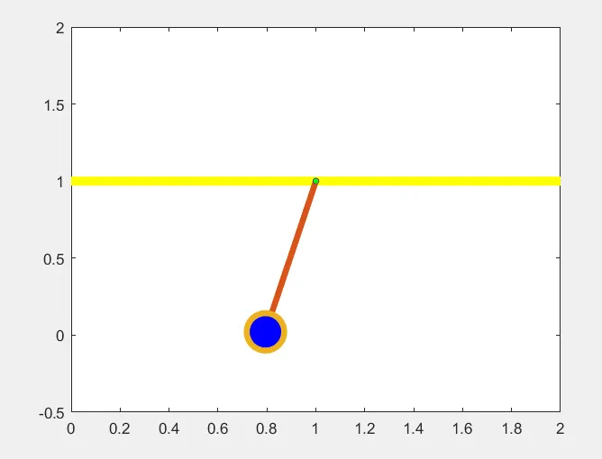
3. Animated file-

https://youtu.be/j4LW8Br4F-I

Conclusion:-

1.The graph of displacement and angular velocity is plotted in graph.

2.Animation of simple pendulum is created.