week-4 Curve fitting
Aim:-
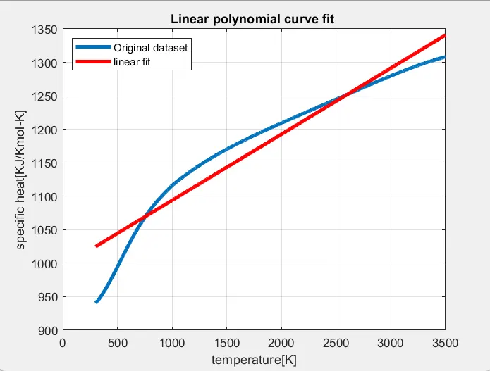
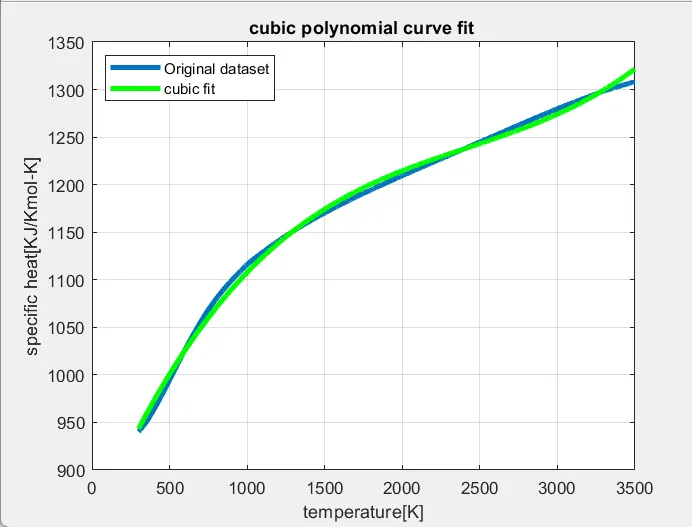
- Write code to fit a linear and cubic polynomial for the Cp data.
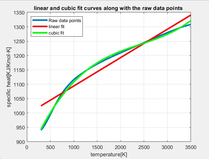
- Plot the linear and cubic fit curves along with the raw data points.
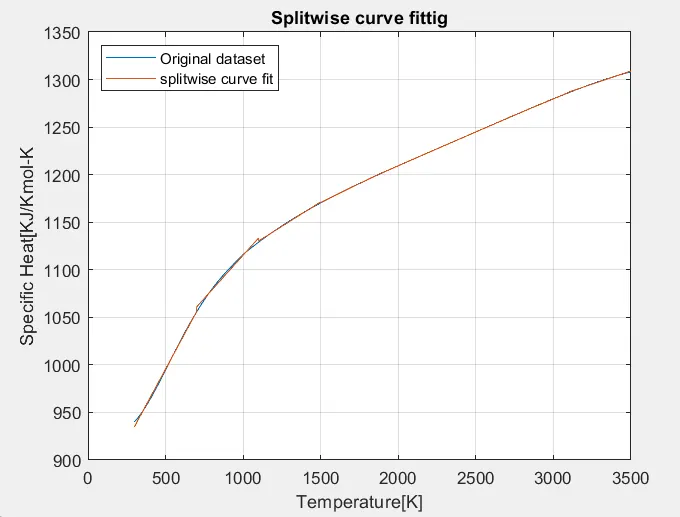
- Write a code to show splitwise method.
- measure the fitness characteristics for both the curves.
Theory:-
Goodness-of-Fit Statistics
After using graphical methods to evaluate the goodness of fit, you should examine the goodness-of-fit statistics. Curve Fitting Toolbox™ software supports these goodness-of-fit statistics for parametric models:
-
The sum of squares due to error (SSE)
-
R-square
-
Adjusted R-square
-
Root mean squared error (RMSE)
For the current fit, these statistics are displayed in the Results pane in the Curve Fitter app. For all fits in the current curve-fitting session, you can compare the goodness-of-fit statistics in the Table Of Fits pane.
To examine goodness-of-fit statistics at the command line, either:
-
In the Curve Fitter app, export your fit and goodness of fit to the workspace. On the Curve Fitter tab, in the Export section, click Export and select Export to Workspace.
-
Specify the
gofoutput argument with thefitfunction.
Sum of Squares Due to Error
This statistic measures the total deviation of the response values from the fit to the response values. It is also called the summed square of residuals and is usually labeled as SSE.
SSE=n∑i=1wi(yi−ˆyi)2
A value closer to 0 indicates that the model has a smaller random error component, and that the fit will be more useful for prediction.
R-Square
This statistic measures how successful the fit is in explaining the variation of the data. Put another way, R-square is the square of the correlation between the response values and the predicted response values. It is also called the square of the multiple correlation coefficient and the coefficient of multiple determination.
R-square is defined as the ratio of the sum of squares of the regression (SSR) and the total sum of squares (SST). SSR is defined as
SSR=n∑i=1wi(ˆyi−‾y)2
SST is also called the sum of squares about the mean, and is defined as
SST=n∑i=1wi(yi−‾y)2
where SST = SSR + SSE. Given these definitions, R-square is expressed as
R-square=SSRSST=1−SSESST
R-square can take on any value between 0 and 1, with a value closer to 1 indicating that a greater proportion of variance is accounted for by the model. For example, an R-square value of 0.8234 means that the fit explains 82.34% of the total variation in the data about the average.
If you increase the number of fitted coefficients in your model, R-square will increase although the fit may not improve in a practical sense. To avoid this situation, you should use the degrees of freedom adjusted R-square statistic described below.
Note that it is possible to get a negative R-square for equations that do not contain a constant term. Because R-square is defined as the proportion of variance explained by the fit, if the fit is actually worse than just fitting a horizontal line then R-square is negative. In this case, R-square cannot be interpreted as the square of a correlation. Such situations indicate that a constant term should be added to the model.
Degrees of Freedom Adjusted R-Square
This statistic uses the R-square statistic defined above, and adjusts it based on the residual degrees of freedom. The residual degrees of freedom is defined as the number of response values n minus the number of fitted coefficients m estimated from the response values.
v = n – m
v indicates the number of independent pieces of information involving the n data points that are required to calculate the sum of squares. Note that if parameters are bounded and one or more of the estimates are at their bounds, then those estimates are regarded as fixed. The degrees of freedom is increased by the number of such parameters.
The adjusted R-square statistic is generally the best indicator of the fit quality when you compare two models that are nested — that is, a series of models each of which adds additional coefficients to the previous model.
adjusted R-square=1−SSE(n−1)SST(v)
The adjusted R-square statistic can take on any value less than or equal to 1, with a value closer to 1 indicating a better fit. Negative values can occur when the model contains terms that do not help to predict the response.
Root Mean Squared Error
This statistic is also known as the fit standard error and the standard error of the regression. It is an estimate of the standard deviation of the random component in the data, and is defined as
RMSE=s=√MSE
where MSE is the mean square error or the residual mean square
MSE=SSEv
Just as with SSE, an MSE value closer to 0 indicates a fit that is more useful for prediction.
How to make a curve fit perfectly?
- For make a curve fit perfectly we can increse the order of polynomial , by increasing the order of polynomial the predicted data curve going towards original data curve.
How to get the best fit?
-To get best fit the value of R_square is > 0.955 , then it is called is best fit.
- if R^2 is 0 then it is called as wrost fit.
- if R^2 is 1 then it is called as best possible fit.
What could be done to improve the cubic fit?
- By splitwise method we can improve the cubic fit.
Program:-
Matlab code to fit linear and cubic polynomial for the given cp data:
% Curve fit for cp data linear and cube polynomial
clear all
close all
clc

% Preparing the data
 cp_data = load('data');
 temperature = cp_data(:,1);                          % Temperature [K]
          cp = cp_data(:,2);                          % specific heat [KJ/Kmol-K]

% linear polynomial curve fit
figure (1)
% cp = a*T+b
co_efficient1 = polyfit(temperature,cp,1);            % coefficient of polynomial are generated
predicted_cp1 = polyval(co_efficient1,temperature);   % predicted values of cp_1 are generated

% compare curve fit with original data
plot(temperature,cp,'linewidth',3)                    % original data set
hold on
plot(temperature,predicted_cp1,'linewidth',3,'color','r')
xlabel('temperature[K]')
ylabel('specific heat[KJ/Kmol-K]')
legend('Original dataset','linear fit','Location','northwest')
title('Linear polynomial curve fit ')
grid on

% Cubic polynomial curve fit
% cp = a*T^3+b*T^2+c*T+d
figure(2)
co_efficient2 = polyfit(temperature,cp,3);
predicted_cp2 = polyval(co_efficient2,temperature);

plot(temperature,cp,'linewidth',3)
hold on
plot(temperature,predicted_cp2,'linewidth',3,'color','g')
xlabel('temperature[K]')
ylabel('specific heat[KJ/Kmol-K]')
legend('Original dataset','cubic fit','Location','northwest')
title('cubic polynomial curve fit ')
grid on

% Curve for linear and cubic fit curves along with the raw data points.
figure(3)
plot(temperature,cp,'linewidth',3)
hold on
plot(temperature,predicted_cp1,'linewidth',3,'color','r')
plot(temperature,predicted_cp2,'linewidth',3,'color','g')
xlabel('temperature[K]')
ylabel('specific heat[KJ/Kmol-K]')
legend('Raw data points','linear fit','cubic fit','Location','northwest')
title('linear and cubic fit curves along with the raw data points ')
grid on

% Calculating goodnes of curve
% to find error
% R_square = SSR/SST

mean = sum(cp)/length(cp);

SSR1 = sum((predicted_cp1-mean).^2);
SSR2 = sum((predicted_cp2-mean).^2);

SSE1 = sum((cp-predicted_cp1).^2);
SSE2 = sum((cp-predicted_cp2).^2);

% SST = SSR+SSE

SST1 = SSR1 + SSE1;
SST2 = SSR2 + SSE2;

R_square1 = SSR1/SST1
R_square2 = SSR2/SST2
Matlab code to show splitwise method:
% Code for splitwise curve fitting
clear all
close all
clc

% Preparing the data
 cp_data = load('data');
 temperature = cp_data(:,1); % Temperature [K]
          cp = cp_data(:,2); % specific heat [KJ/Kmol-K]

plot(temperature,cp)
hold on

% Splittting the data into 4 data folds
 a = 1;
 b = 400;

 for i = 1:8
     co_efficient = polyfit(temperature(a:b),cp(a:b),1);
     predicted_cp(a:b,1) = polyval(co_efficient,temperature(a:b));
     a = b+1;
     b = b+400;
 end

plot(temperature,predicted_cp)
title('Splitwise curve fittig')
xlabel('Temperature[K]')
ylabel('Specific Heat[KJ/Kmol-K')
legend('Original dataset','splitwise curve fit','Location','northwest')
grid on

% Calculating goodnes of curve
% to find error
% R_square = SSR/SST

mean = sum(cp)/length(cp);

SSR = sum((predicted_cp-mean).^2);
SSE = sum((cp-predicted_cp).^2);

% SST = SSR+SSE

SST = SSR + SSE;

R_square1 = SSR/SST
Explanation of code:-
*clera all- To clear all variables from current workplace.
*close all- close all figures whose handles are visible.
*clc - clc clears all the text from the command window.
* load()- load command read the entire contents of the file in a single step. The load command requires that the data in the file be organized into a rectangular array.
*ployfit()-This MATLAB function returns the coefficients for a polynomial p(x) of degree n that is a best fit (in a least-squares sense) for the data in y.
*polyval()-This MATLAB function evaluates the polynomial p at each point in x.
*plot()- creates a 2-D line plot .
*hold on -retains the current plot and certain axes properties so that subsequent graphing commands add to the existing graph.
*xlabel()- It labels the x-axis of the current plot.
*ylabel()- It labels the y-axis of the current plot.
*legend()-legend creates a legend with descriptive labels for each plotted data series.
*title()- add a title to a plot.
*grid on- It displays grid lines.
Results:-
Linear polynomial curve fit plot -
cubic polynomial curve fit plot -
Linear and cubic fit curves along with the raw data points-
Linear splitwise curve fitting plot -
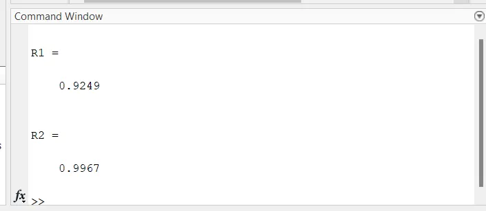
Evaluation of Goodness of Fit -
For Linear and cubic fit:
For Linear splitwise curve fit:
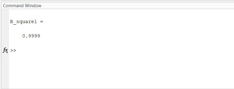
Higher the value of R_square , the better is the curve .
In the case of linear splitwise curve fit the value of R_square is 0.999 then the obtained fit is best fit
Conclusion:-
We get linear and cubic polynomial fit plot for the given Cp data.
We get Linear and cubic fit curves along with the raw data points.
The error is minimized by splitwise curve fitting using linear polynomial.
References:-
https://in.mathworks.com/help/curvefit/evaluating-goodness-of-fit.html
https://projects.skill-lync.com/projects/Curve-Fitting-and-criterion-to-choose-best-fit-41860