Week 4.1 - Genetic Algorithm
Aim:- Optimise the stalagmite function and find the global maxima of the function using Matlab.
Introduction to GA ( Genetic algorithm ):-
The genetic algorithm is a method for solving both constrained and unconstrained optimization problems that is based on natural selection, the process that drives biological evolution. The genetic algorithm repeatedly modifies a population of individual solutions. At each step, the genetic algorithm selects individuals from the current population to be parents and uses them to produce the children for the next generation. Over successive generations, the population "evolves" toward an optimal solution. You can apply the genetic algorithm to solve a variety of optimization problems that are not well suited for standard optimization algorithms, including problems in which the objective function is discontinuous, nondifferentiable, stochastic, or highly nonlinear. The genetic algorithm can address problems of mixed integer programming, where some components are restricted to be integer-valued.
Syntax for ga in MATLAB:-
x = ga(@fun,nvars,A,b,Aeq,beq,lb,ub,nonlcon,intcon,options)
where-
@fun = function handle
nvars = Number of variables
A,b = Linear inequality constraints
Aeq,beq= Linear equality constraints
lb,ub = Lower bounds, Upper bounds
nonlcon = Nonlinear constraints
intcon = Integer variables
options = Optimization options
Matlab code:-
Code for stalagmite function and find the global maxima -
Function code -
function  [f] = stalagmite(input_vector)
x= input_vector(1);
y= input_vector(2);

f1_x = (sin(5.1*pi*x+0.5))^6;
f1_y = (sin(5.1*pi*y+0.5))^6;

f2_x = exp(-4*log(2)*((x-0.0667)^2/0.64));
f2_y = exp(-4*log(2)*((y-0.0667)^2/0.64));

f = -(f1_x*f1_y*f2_x*f2_y);        % -ve for finding global maxima
end
Main code -
clear all
close all
clc

% Defining our search space
x = linspace(0,0.6,150);
y = linspace(0,0.6,150);

% Creating 2d Dimensional mesh
[xx,yy] = meshgrid(x,y);

% Evaluating the stalagmite function

for i = 1:length(xx)
    for j =1:length(yy)
        input_vector(1)=xx(i,j);
        input_vector(2)=yy(i,j);
        f(i,j) = stalagmite(input_vector);
    end
end
surfc(xx,yy,f)
xlabel('xvalue')
ylabel('yvalue')
title('Stalagmite mathematical model')
shading interp
[inputs,fval] = ga(@stalagmite,2)
Code for all 3 studies of stalagmite function -
Function code -
function [f]=get_stalagmite(x,y)
  [x y] =meshgrid(x,y);

for i=1:length(x);
    for j=1:length(y);
        input_vector(1) =x(i,j);
        input_vector(2) =y(i,j);
        f(i,j)=stalagmite(input_vector);
    end
end

end
Main code -
clear all
close all
clc

% Defining our search space
x = linspace(0,0.6,150);
y = linspace(0,0.6,150);
[xx,yy] = meshgrid(x,y);
num_cases=50;
f=get_stalagmite(x,y);
tic
% Study 1 - Stastical Behavior
for i =1:num_cases
    [inputs,fopt(i)]=ga(@stalagmite,2);
    xopt(i)=inputs(1);
    yopt(i)=inputs(2);
end
study1_time =toc
figure(1)
subplot(2,1,1)
hold on
surfc(x,y,f)
shading interp
plot3(xopt,yopt,fopt,'marker','o','markersize',5,'markerfacecolor','r')
title('unbounded inputs')
subplot(2,1,2)
plot(fopt)
xlabel('iterations')
ylabel('Function maximum')

tic
% Study 2 - Stastical behavior with upper and lower bonds.

for i =1:num_cases
    [inputs,fopt(i)]=ga(@stalagmite,2,[],[],[],[],[0;0],[0.6;0.6]);
    xopt(i)=inputs(1);
    yopt(i)=inputs(2);
end
study2_time =toc
figure(2)
subplot(2,1,1)
hold on
surfc(x,y,f)
shading interp
plot3(xopt,yopt,fopt,'marker','o','markersize',5,'markerfacecolor','r')
title('bounded inputs')
subplot(2,1,2)
plot(fopt)
xlabel('iterations')
ylabel('Function maximum')

% Study 3 - Increasing GA iterations

options = optimoptions('ga');
options = optimoptions(options,'PopulationSize',170);
tic
for i =1:num_cases
    [inputs,fopt(i)]=ga(@stalagmite,2,[],[],[],[],[0;0],[0.6;0.6],[],[],options);
    xopt(i)=inputs(1);
    yopt(i)=inputs(2);
end
study3_time =toc
figure(3)
subplot(2,1,1)
hold on
surfc(x,y,f)
shading interp
plot3(xopt,yopt,fopt,'marker','o','markersize',5,'markerfacecolor','r')
title('bounded inputs with modified population size')
subplot(2,1,2)
plot(fopt)
xlabel('iterations')
ylabel('Function maximum')
Code explations:-
*clera all- To clear all variables from current workplace.
*close all- close all figures whose handles are visible.
*clc - clc clears all the text from the command window.
*linspace()- This function will generate a vector of values linearly spaced between two endpoints.
*meshgrid()- It is used to create rectangular structures from the given arrays which represent the indexing in the matrix.
*surfc()-This is used to plot a surface plot that is three-dimensional in nature and a contour plot underneath of it.
*plot()- creates a 2-D line plot .
*xlabel()- It labels the x-axis of the current plot.
*ylabel()- It labels the y-axis of the current plot.
*title()- add a title to a plot.
*shading inturp - this command is used for remove the grid lines from the face of plot.
*ga(@fun,nvars) - its a inbuilt genetic algorithm matlab solver for use the solving functions.
*subplot- It divides the current figure into rectangular panes that are numbered row-wise. Each pane contains an axes. Subsequent plots are output to the current pane.
*hold on -retains the current plot and certain axes properties so that subsequent graphing commands add to the existing graph.
Results:-
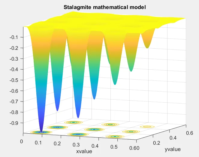
here we obtained the value of Function maximum =0.4971
Study 1 - Stastical Behavior (Unbounded)
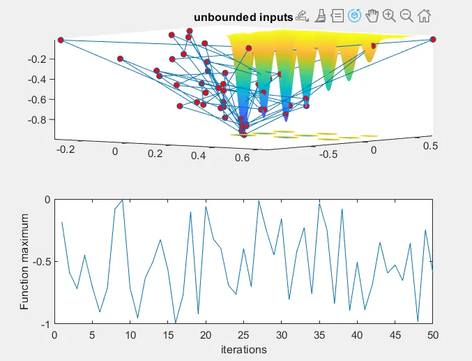
Study time-3.4479
Study 2 - Stastical behavior with upper and lower bonds-
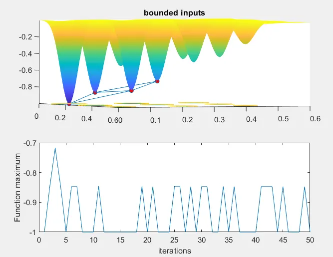
Study time-4.2263
Study 3 - Increasing GA iterations (Population size)-
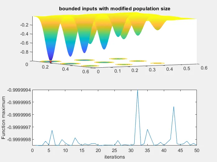
Study time-7.9267
References:-