Project 1
AIM: to get familiar with the modeling process, writing scripts in Matlab, modeling in Simulink, analyzing data and generating plots.
OBJECTIVES:
The task of this project is to compute the fuel economy numbers for the given vehicle (kmpl) on the urban cycle (UDDS) and highway cycle (HWFET). Also, to analyze and understand the vehicle operating
points in terms of engine speed, torque, transmission speeds, pedal positions, gear, distance traveled, etc.
1) Load the Project1 folder as the Current Folder in Matlab.
2) Run the “Project1_InitFile.m” Matlab script.
3) The provided vehicle Simulink model “Project1_VehicleModel.slx” is incomplete. The engine and vehicle dynamics block contents have been deleted. Build the Simulink blocks by referring to the course lecture and example block images provided. You can run the model and analyze the results using a ‘Scope’ for debugging.
4) Add additional ‘To Workspace’ blocks for transferring the desired Simulink vehicle data into the Matlab workspace.
5) Modify the “Project1_ProcessingFile.m” as per the desired plots and required calculations.
6) Write a project report that contains the following:
a. Tabulate the fuel economy numbers (kmpl) for UDDS and HWFET cycle. This forms the baseline numbers for comparing with the future hybrid version.
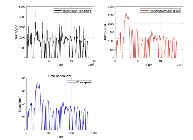
b. Plot the time trace for engine, transmission input, transmission output and wheel speed on one plot.
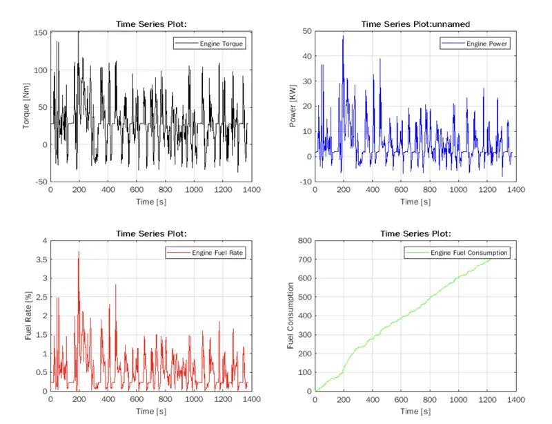
c. Plot engine torque, engine power, fuel rate and fuel consumption using subplots.
d. Plot accelerator and brake pedal, gear command, vehicle desired and actual speed, vehicle distance using subplots.
e. Plot the engine operating points on the engine fuel map.
f. Write down appropriate brief comments on each of these plots, describing the vehicle behavior throughout the drive cycle.
g. Generate the plots for both drive cycles
PROCEDURE:
- firstly we have loaded the Project1 folder in MATLAB
- then we have run the Project1_InitFile.m in the MATLAB script
- then we have made some adjustments in the file as per our desires to get thee results we want out of this challenge
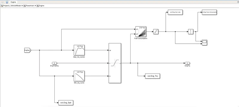
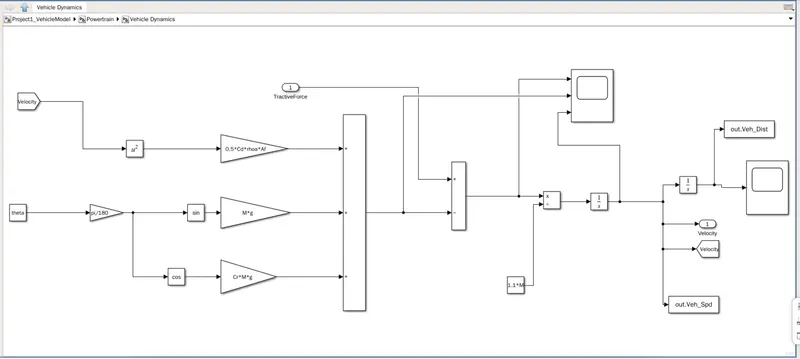
- Then we have completed the Engine and the Vehicle Dynamics blocks in Simulink
- Also we have added certain "to Workspace" blocks to load desired values into our MATLAB workspace
- then we ran the SIMULINK model and all the "to Workspace Block" Values are transferred to MATLAB WORKSPACE>
- Then we made some adjustment in the plot section of Project1_ProcessingFile.m and then ran the file 2 times
- First one is for UDDS drive cycle and the Second one is for HWFET drive cycle
- In the Project1_ProcessingFile.m we made the following adjustments
- Plotted the time trace for engine, transmission input, transmission output and wheel speed on one plot.
- Plotted engine torque, engine power, fuel rate and fuel consumption using subplots.
- Plotted accelerator and brake pedal, gear command, vehicle desired and actual speed, vehicle distance using subplots.
- Plotted the engine operating points on the engine fuel map.
Coding:
CHANGES MADE IN "PROJECT1_INITFILE.M"
%%%%%%%%%%%%%%%%%%%%%%%%%%%%%%%%%%%%%%%%%%%%%%%%%%%%%%%%%%%%%%%%%%%%%
%% Skill-Lync -> Hybrid Drives Development
% Project 1 - Conventional Vehicle Model
% By - Ullekh Gambhira

% Description:

%% Initialization File
% Initialization file for loading the variables for the Conventional vehicle simulation model

%% Vehicle Parameters
M = 1500;       % Vehicle weight [kg]
Cr = 0.015;     % Rolling resistance coefficient
Rw = 0.35;      % Rolling radius [m]
Cd = 0.33;      % Drag coefficient
Af = 2;         % Frontal area [m2]
rhoa = 1.225;   % Air density [kg/m3]
Vwind = 0;      % Wind velocity [kmph]
g = 9.81;       % Gravitational acceleration [m/s2]
theta = 0;      % Slope [deg]
myu_road_tire = 1; % Coefficient of friction between tire - road interface

Tm = 150;       %motor torque [nm]
efft = 0.8;     %transmission efficiency
ratio =2.45;    %Total ratio

%vehicle top speed
Vveh = sqrt(efft*ratio/Rw*Tm - Cr*M*g)*2/rhoa/Af/Cd;  %vehicle velocity in[m/s]
Vveh_kmph = Vveh*18/5;                               %vehicle velocity in[kmph]

%power for top speed
Fload = (0.5*Cd*rhoa*Af*(Vveh + Vwind)^2) + Cr*M*g*cosd(theta) + M*g*sind(theta); %road load in[N]
Pload = Fload*Vveh/1000;         %road load power in[Kw]

%powertrain speed
omegam = ratio*Vveh/Rw;          %motor speed in [rad/sec]
omegam_rpm = omegam*30/pi;       %motor speed in[rpm]


%% Powertrain Parameters
FDR = 3.73;                         % Final Drive Ratio / Diff Ratio
DiffEff = 0.99;                     % Differential efficiency (assumed independent of operating conditions)

NumGear = 4;                        % Number of gears in transmission
TransGear = [1:NumGear];            % Transmission Gears
TransRatio = [3.06, 1.62, 1, 0.7];  % Corresponding Transmission ratios
TransEff = 0.90;                    % Transmission efficiency (assumed independent of operating conditions)

TC_SR = [0, .5, .6, .7, .8, .87, .92, .94, .96, .97, 1];   % Torque Converter Speed Ratio (Matlab default) -> TurbSpd/PumpSpd
TC_TR = [2.232, 1.5462, 1.4058, 1.2746, 1.1528, 1.0732, 1.0192, 1, 1, 1, 1];   % Torque Converter Torque Ratio (Matlab default) -> TurbTrq/PumpTrq
TC_Cf = 1e-4 * [.72558, .66322, .63463, .59042, .51331, .4144, .29287, .22444, .12186, .04386, 0]; % Torque Converter Capacity Factor (Matlab default) -> PumpTrq/PumpSpd^2 [Nm/rpm^2]

load Vehicle_Data/Engine_data_1_9L_Saturn_95kW
load Vehicle_Data/Trans_Shift_map

%% Driver Parameters
Kp = 10;                    % P gain for driver PI model
Ki = 1;                     % I gain for driver PI model
Drive_Cycle_Select = 1;     % Drive cycle selection

% Drive cycle values in m/s

if Drive_Cycle_Select == 1
    load DriveCycles/UDDS.MAT;

elseif Drive_Cycle_Select == 2
    load DriveCycles/HWFET.mat;

elseif Drive_Cycle_Select == 3
    load DriveCycles/FTP;

elseif Drive_Cycle_Select == 4
    load DriveCycles/US06;

elseif Drive_Cycle_Select == 5
    load DriveCycles/NEDC;

elseif Drive_Cycle_Select == 6
    load DriveCycles/WLTP;

end

time_end = cyc_time(end);
vel_end = cyc_vel(end);
CHANGES MADE IN "PROJECT1_PROCESSING.M"
%%%%%%%%%%%%%%%%%%%%%%%%%%%%%%%%%%%%%%%%%%%%%%%%%%%%%%%%%%%%%%%%%%%%%
%% Skill-Lync -> Hybrid Drives Development
% Project 1 - Conventional Vehicle Model
% By - Ullekh Gambhira

% Description:
% The following file is to used with the Initialization file and Simulink
% results for post-processing of the data.
% The file is incomplete, has some examples of how the data is imported
% into a readable format, data analysis and plotting examples.
% Based on the project task, use commands in a similar format as given
% below, to analyse the data and generate required plots.
% You can change variable names if desired

%% Post-Processing File
%  File for post-processing the Conventional vehicle simulation model data

%% Renaming variables
Time = out.tout;
Acc_Pdl = out.Acc_Pdl;          % Accelerator pedal [%]
Brk_Pdl = out.Brk_Pdl;          % Brake pedal [%]
Gear_Cmd = out.Gear_Cmd;        % Transmission gear
Trans_In_Spd = out.Trans_In_Spd*30/pi;  % Transmission input speed [rpm]
Trans_Out_Spd = out.Trans_Out_Spd*30/pi;% Transmission output speed [rpm]
Eng_Trq = out.Eng_Trq;          % Engine brake torque [Nm]
Eng_Spd = out.Eng_Spd*30/pi;    % Engine speed [rpm]
Eng_Fuel_Consump = out.Eng_Fuel_Consumption;    % Engine fuel consumption [g]
Veh_Dist = out.Veh_Dist/1000;   % Distance traveled by vehicle [km]
Veh_Spd = out.Veh_Spd*18/5;     % Vehicle speed [kmph]
Wheel_Spd = out.WhSpd;          %Wheel speed in[kmph]
Eng_Fuel_Rate = out.Eng_fuel_rate;

%% Data Analysis
Eng_Pwr = Eng_Spd*pi/30*Eng_Trq/1000;   % Engine brake power [kW]
rho_petrol = 0.7197;                    % Density of petrol [kg/L]
kmpl = Veh_Dist(end)/(Eng_Fuel_Consump(end)/1000/rho_petrol);    % Fuel economy [kmpl]


%% Plotting vehicle characteristics time trace
figure(1)
subplot(3,1,1)
hold on
grid on
plot(Time, Acc_Pdl,'linewidth',1,'Color','black');
plot(Time, Brk_Pdl,'linewidth',1,'Color','red');
ylabel('Pedal [%]')
xlim([0, Time(end)]);
legend('Accel','Brake');
subplot(3,1,2)
hold on
grid on
plot(Time,Trans_In_Spd,'linewidth',1,'Color','black');
plot(Time,Trans_Out_Spd,'linewidth',1,'Color','red');
ylabel('Speed [rpm]')
xlim([0, Time(end)]);
ylim([0, 6000]);
legend('Trans Input','Trans Output');
subplot(3,1,3)
hold on
grid on
plot(Time, Gear_Cmd,'linewidth',1,'Color','black');
xlim([0, Time(end)]);
xlabel('Time [s]');
ylabel('Gear');

%% Plotting engine operating points on engine fuel map
figure()
figure('Name','Engine Operating Points');
hold on
grid on
title('Engine Operating Points','fontsize',12);
p1=plot(Eng_map_spd*30/pi,Eng_max_trq,'linewidth',2,'color','r');
p2=line([Eng_map_spd(end)*30/pi Eng_map_spd(end)*30/pi],[0 Eng_max_trq(end)]);
set(p2,'linewidth',1,'linestyle','--','color','k');
p3=line([Eng_map_spd(1)*30/pi Eng_map_spd(1)*30/pi],[0 Eng_max_trq(1)]);
set(p3,'linewidth',1,'linestyle','--','color','k');
[c,h] = contour(Eng_map_spd'*30/pi,Eng_map_trq,Eng_fuel_map');
clabel(c,h);
xlabel('Engine Speed [rpm]');
ylabel('Engine Torque [Nm]');
title('Engine Fuel Consumption Map [g/s]');
% p4 = plot(Eng_Spd,Eng_Trq,'.','color','k');
% legend([p1 p4],{'Max Curve','Operating Points'});
% axis([Eng_map_spd(1)*30/pi Eng_map_spd(end)*30/pi 0 Eng_map_trq(end)]);


%plotting engine torque, engine power, fuel rate and fuel consumption using subplots.
subplot(2,2,1)
plot(Eng_Trq,'linewidth',1,'color','black')
xlabel('Time [s]')
ylabel('Torque [Nm]')
legend('Engine Torque')
grid on
subplot(2,2,2)
plot(Eng_Pwr,'linewidth',1,'color','blue')
xlabel('Time [s]')
ylabel('Power [KW]')
legend('Engine Power')
grid on
subplot(2,2,3)
plot(Eng_Fuel_Rate,'linewidth',1,'color','red')
xlabel('Time [s]')
ylabel('Fuel Rate [%]')
legend('Engine Fuel Rate')
grid on
subplot(2,2,4)
plot(Eng_Fuel_Consump,'linewidth',1,'color','green')
xlabel('Time [s]')
ylabel('Fuel Consumption')
legend('Engine Fuel Consumption')
grid on

%plotting the time trace for engine, transmission input, transmission output and wheel speed
figure()
subplot(2,2,1)
title('Time Traces','fontsize',12);
plot(Trans_In_Spd, 'linewidth', 1, 'Color', 'black');
xlabel('Time');
ylabel('Trans_In_Spd')
legend('Transmission input speed')
grid on
subplot(2,2,2)
plot(Trans_Out_Spd, 'linewidth', 1, 'Color', 'red');
xlabel('Time')
ylabel('Trans_Out_Spd')
legend('Transmission output speed');
grid on
subplot(2,2,3)
plot(Wheel_Spd, 'linewidth',1, 'color', 'blue');
legend('Wheel speed')
ylabel('Speed [rpm]')
xlabel('Time');
grid on

% Plotting fuel economy Vs Engine Fuel consumption
figure()
plot(Eng_Fuel_Rate,'color','r')
plot(Eng_Fuel_Consump,'color','b')
xlabel('Fuel consumption')
ylabel('Fuel Rate [%]')
title('Fuel economy Vs Fuel Consumption')
grid on
CHANGES MADE IN SIMULINK MODEL
ENGINE BLOCK
VEHICLE DYNAMICS BLOCK
RESULTS:
- FOR UDDS DRIVE CYCLE
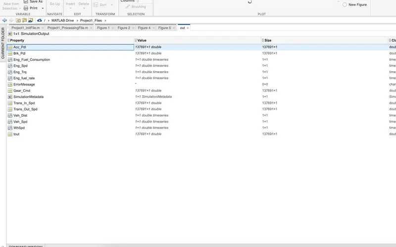
WORKSPACE DETAILS
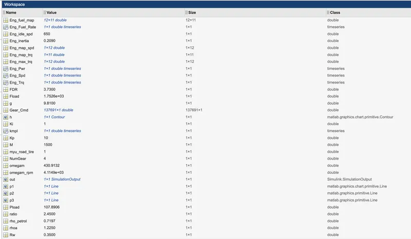
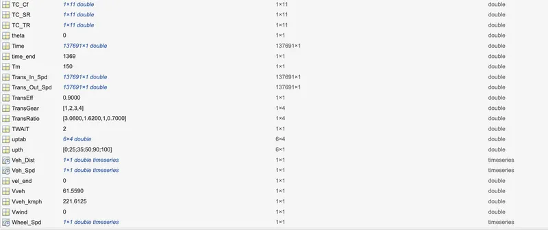
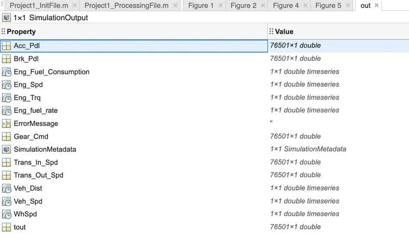
WORSPACE DETAILS FOR "TO WORSPACE" BLOCKS USED IN THE MODEL
NOW FOR THE PLOTS:
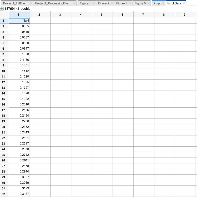
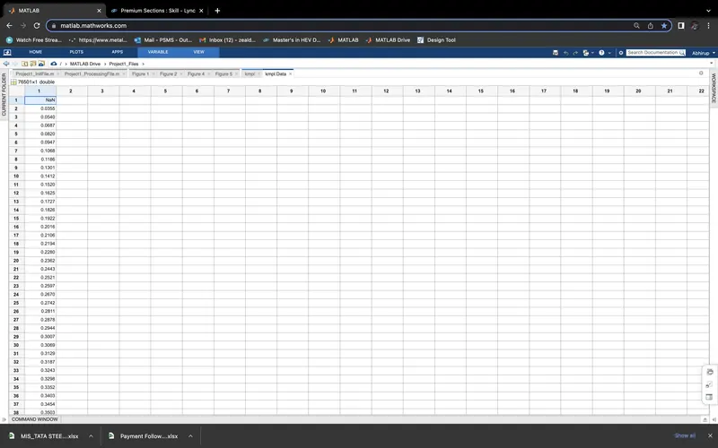
a. KMPL DATA UDDS DRIVE CYCLE
b.Plot the time trace for transmission input, transmission output and wheel speed on one plot.
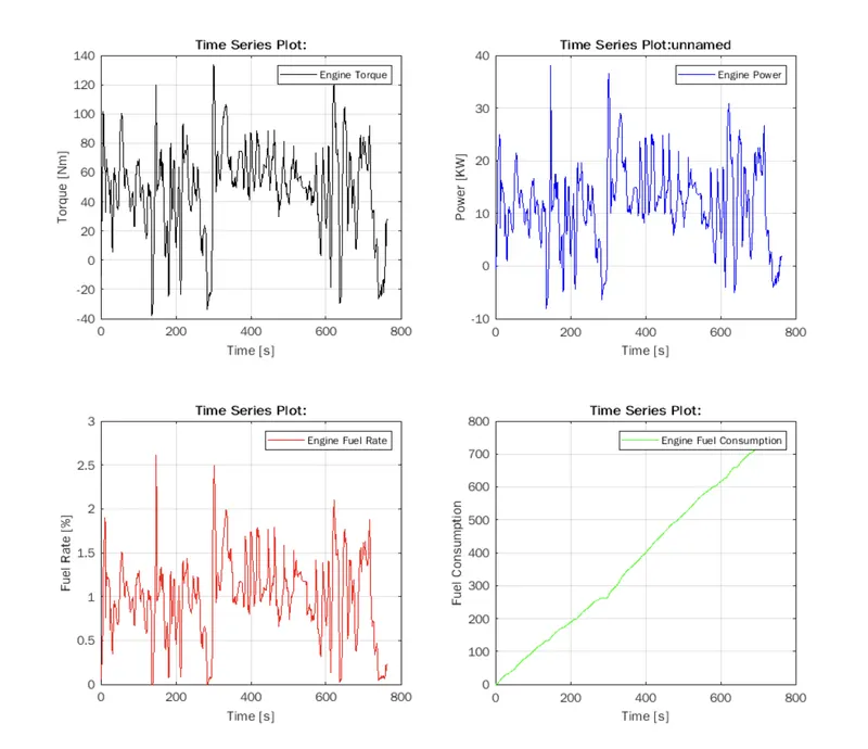
c.Plot engine torque, engine power, fuel rate and fuel consumption using subplots.
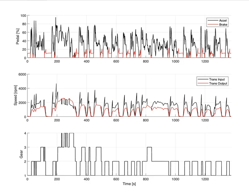
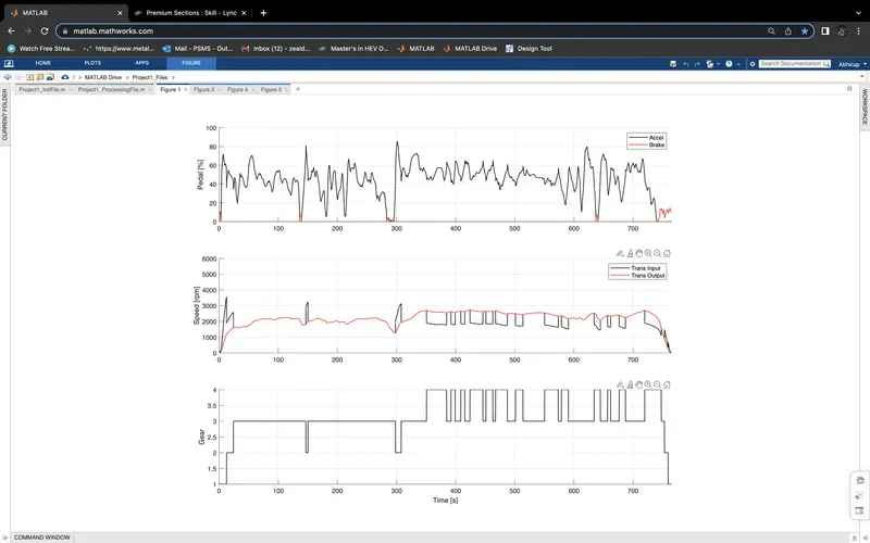
d. Plot accelerator and brake pedal, gear command, vehicle desired and actual speed, vehicle distance using subplots.
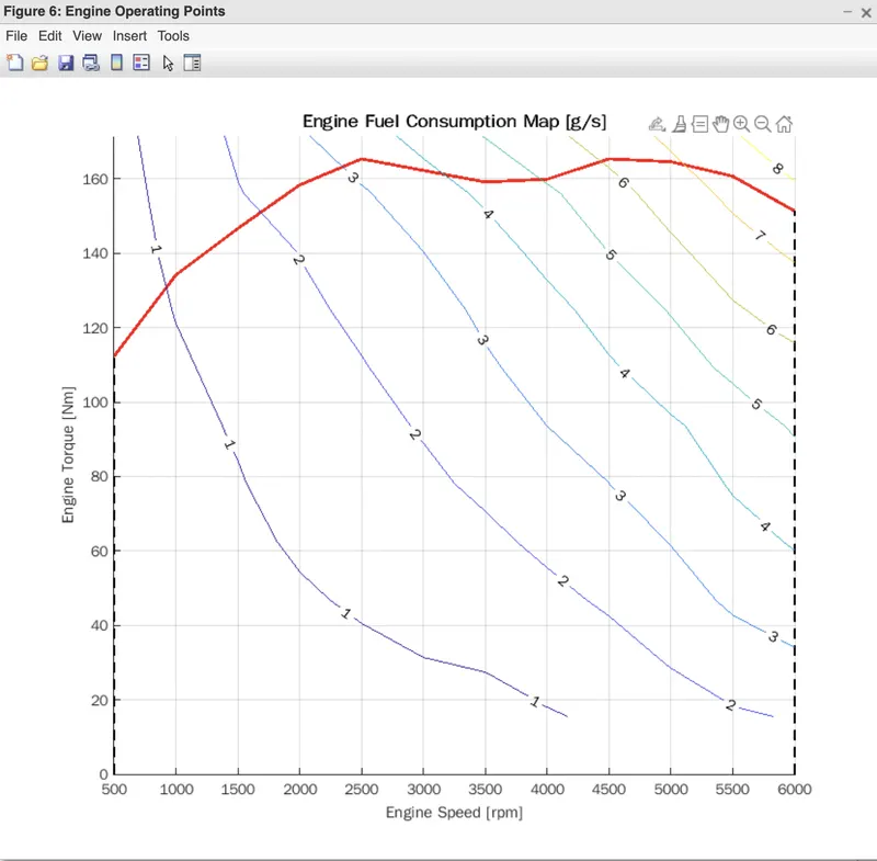
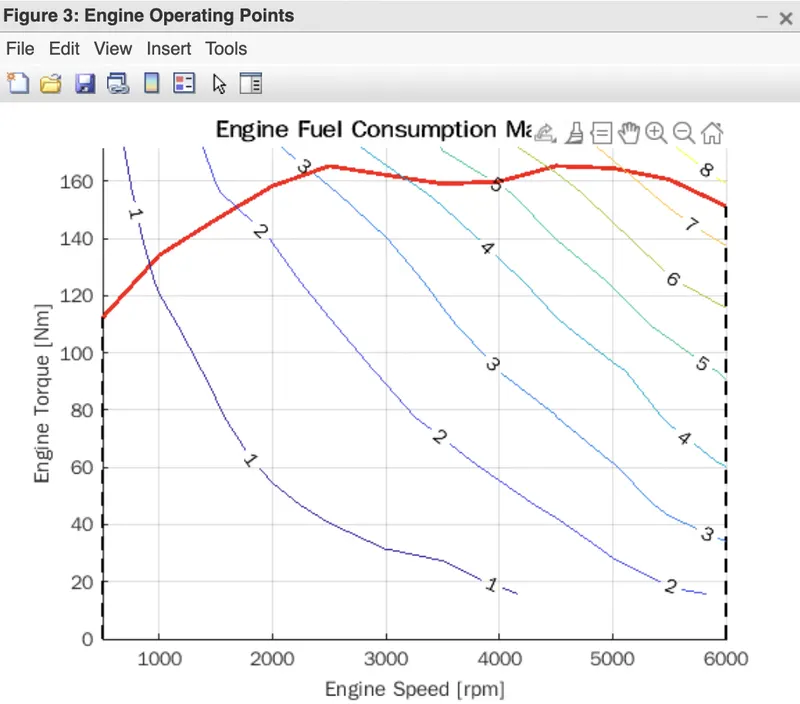
e. Plot the engine operating points on the engine fuel map.
REMARKS AND COMMENTS FOR EACH PLOT:
PLOT D:
- HERE WE CAN SEE IN THE ACCELERATOR PEDAL AND BRAKE PEDAL PLOT, WHENEVER THE DRIVER PUSHES THE BRAKE PEDAL, THE ACCELARATION OF THE VEHICLE DECREASES AND THE VEHICLE DECELARATES.
- SIMILARLY FOR THE TRANSMISIION INPUT AND OUTPUT, WHENEVER THE DRIVER PUSHES THE BRAKES, THE TRANSMISSION FOR THE VEHICLE SHARPLY DECREASES AS THIS IS A CITY RIDE TEST AND THE VEHICLE DECELARATES AND COMES TO A TEMPORARY HALT.SIMILARY THE TRANSMISSION OUTPUT BEHAVES THE SAME, PROVIDING 0 TO MINIMUM OUTPUT POWER IN CASE OF BRAKING. WHEN DRIVER HITS THE ACCEL PEDAL, THE TRANSMISSION INPUT POWER RISES STEEPLY IN RISE WITH TRANSMISSION OUTPUT POWER
- THE GEAR COMMAND PLOT ALSO TELLS US THE SAME BEHAVIOR. BY LOOKING AT THE PLOT WE CAN TELL WHENEVER THE DRIVER PUSHES THE BRAKE PEDAL TO STOP THE VEHICLE, IN THE NEXT INSTANT HE HAS TO INCREASE THE GEARS IN ORDER TO OBTAIN MORE SPEED.
PLOT B:
- AS MENTIONED FOR PLOT A, IT IS THE SAME FOR PLOT B.
- IN THIS CASE WE SEE THAT IN 200TH SECOND THE TRSANSMISSION INPUT POWE, THE TRANSMISSION OUTPUT POWER AAND THE WHEEL SPEED OF THE VEHICLE OBTAIN A PEAK VALUE THROUGHT THE WHOLE PLOT WHICH MEANS THAT THE VEHICLE OBTAINS A TOP SPEED OF APPROXIMATELY 75 KMPH DURING THAT TIME.ALSO WE SEE THAT THE DRIVER SLOWS DOWN THE VEHICLE FOR A VERY SHORT AMOUNT OF TIME AND THE SPPED OF THE WHEEL DECREASES A LIITLE BIT THEN AGAIN IT REACHES THE TOP SPEED.
- ON THE OTHER HAND WE SEE THE EFFECT OF BRAKING THROUGHT THE WHOLE PLOT WHERE THE DRIVER BRAKES AND ACCELARATES CONTINOUSLY WHICH INDICATES THE CITY DRIVING CONDITIONS.
- THIS CONSTANT DECELARATING AND ACCELARATING GIVES RISES TO A DROP OF TRAMSMISSION INPUT POWER, TRANSMISSION OUTPUT POWER AND THE WHEEL SPEED.
PLOT C:
- HERE IN THIS PLOT WE CAN SEE THAT THE ENGINE TORQUE REACHES A PEAK POINT AT 200TH SEC WHERE THE POWER OF THE ENGINE GIVES RISE TO THE AMOUNT OF FUEL CONSUMED FROM 200TH SEC AND DECREASES TO A MINIMUM STATE AT ARROUND 350TH SEC.
- HERE IN THE FUEL CONSUMPTION GRAPH WE SEE THAT AS THE VEHICLE MOVES FROWARD THERE IS A CONSTANT CONSUMPTION OF THE FUEL TO THE ENGINE.
- ALSO WE SEE THE CHANGE IN FUEL CONSUMPTION RATES AS THE DRIVER ACCELARATES AND BRAKES.
PLOT E:
- IN THIS PLOT WE BASSICALLY MAP THE FUEL CONSUMPTION OF THE ENGINE OF THE VEHICLE WITH THE ENGINE TORQUE WHICH IS BASICALLY A FUNCTION OF ENGINE SPEED.
-----------------------------------------------------------------------XXXXX------------------------------------------------------------------------------
RESLUTS
FOR HWFET DRIVE CYCLE:
NOTE: to get the HWFET Drive cycle we have changed the drive cycle value to 2
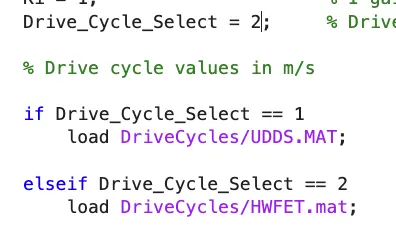
WORKSPACE DETAILS:
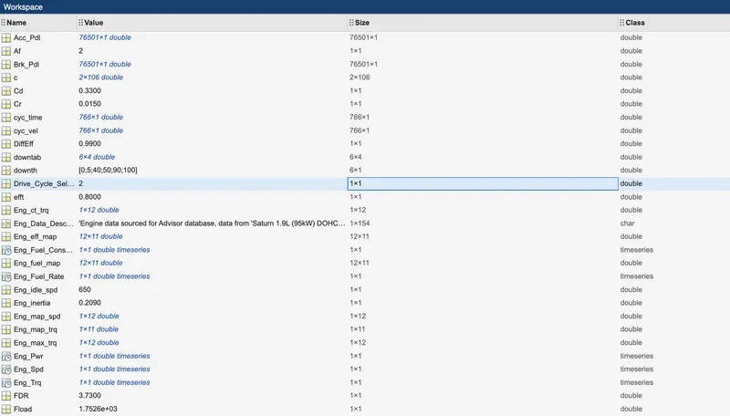
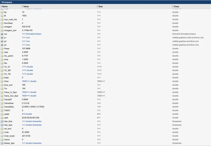
"TO WORKSPACE" BLOCK DETAILS
PLOTS:
A.FUEL ECONOMY NUMBERS(KMPL)
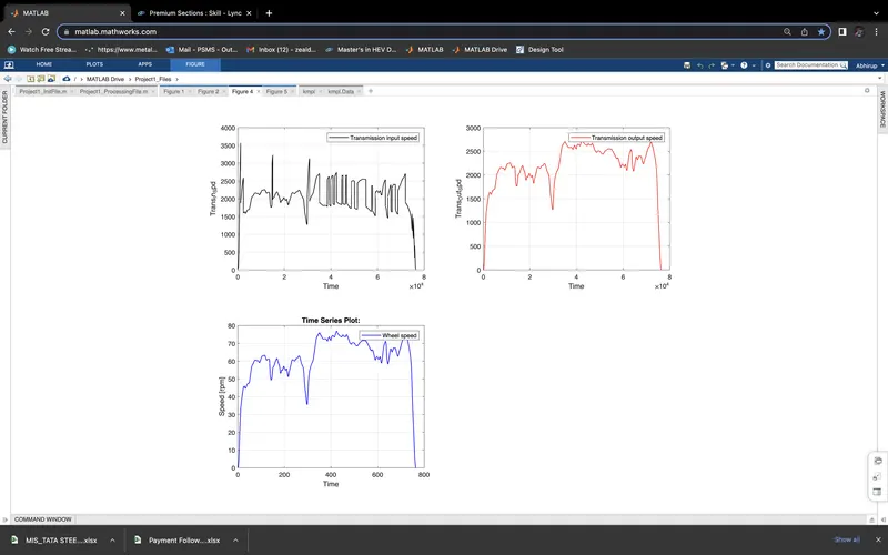
B. Plot the time trace for transmission input, transmission output and wheel speed on one plot.
C.Plot engine torque, engine power, fuel rate and fuel consumption using subplots.
D.Plot accelerator and brake pedal, gear command, vehicle desired and actual speed, vehicle distance using subplots.
E.. Plot the engine operating points on the engine fuel map.
REMARKS AND COMMENTS FOR PLOTS:
PLOT D:
- HERE WE CAN SEE IN THE ACCELERATOR PEDAL AND BRAKE PEDAL PLOT, WHENEVER THE DRIVER PUSHES THE BRAKE PEDAL, THE ACCELARATION OF THE VEHICLE DECREASES AND THE VEHICLE DECELARATES.
- ALSO WE CAN SEE HERE THAT AS THIS IS HIGHWAY DRIVE CYCLE TEST THERFORE THERE SHOULD BE A LOT LESS SUDDEN BRAKINGS COMPARED TO A CITY DRIVE TEST .SO THE PLOT PLOT SHOWS US EXACLTY THE SAME THING, THERE IS DECELERATON BUT THERE IS NO SUDDEN BRAKING.
- JUST AS WE STATED THE ABOVE REASON, THE TRANSMISSION INPUT STAYS STEAY WITH A SLIGHTLY STEADY TRANSMISSION OUTPUT COMPARED TO UDDS DRIVE CYCLE TEST.
- SAME GOES FOR THE GEAR COMMAND PLOT, THE VEHICLE MOVES ON A PARTICULAR GEAR FOR SOME TIME THEN THE DRIVER CHANGES THE GEAR TO INCREASE VEHICLE SPEED.
- MOVING FURTHER IN THE PLOT WE SEE MANY BRAKINGS AND SUDDEN STOPS TO THE VEHICLE ACCELARATION WHICH GIVES RISE TO CHANAGE IN TRANSMISSION INPUT AS WELL AS TRANSMISSION OUTPUT
- AS WELL AS WHEN THERE IS A SUDDEN STOP THE DRIVER REDUCES THE GEAR COMMAND AND INCREASES IT WHEN HE DESIRES SPEED.
PLOT B:
- JUST AS STATED EAERLIER, DUE TO HIGHWAY DRIVE, THER IS A LOT LESS SUDDEN BRAKINGS, SO THE SPEED OF THE VEHICLE IS HIGHER THAN THE UDDS DRIVE CYCLE.
- THIS CAN BE SEEN IF WE HAVE A LOOK AT THE WHEEL SPEED PLOT.
- ALSO THE TRANSMISSION INPUT AND OUTPUT BLOCK GIVES US AN IDEA THAT DUE TO MUCH SMOOTHER TRANSMISSION INPUT THE TRANSMISSION OUTPUT REMAINS HIGHER
PLOT C:
- IN THIS CASE WE HAVE THE ENGINE TORQUE AND ENGINE POWER PLOTS WHICH SHOWS US THE PERFORMANCE OF THE ENGINE OVER TIME AND HOW THE ENGINE HAS ITS POWER OUTPUT.
- THE FUEL CONSUMPTION PLOT OVER TIME IS ALSO PROVIDED TO SHOW THE RATE OF FUEL CONSUMPTION OVERTIME BY THE ENGIN.
- LASTLY WE CAN SEE THE FUEL CONSUMPTION PLOT WHICH SHOWS US THE INCREASE OF FUEL CONSUMED BY THE VEHICE ENGINE TILL HTE END OF THE TEST.
PLOT E:
- AND LASTLY WE HAVE THE ENGINE FUEL CONSUMPTION MAP WHICH HAS THE ENGINE OPERATION POINTS .
CONCLUSION:HERE WE HAVE SUCCESFULLY STUDIED THE COMPARISION OF BOTH UDDS AND HWFET DRIVE CYCLE, THEIR PROPERTIES BY USING VARIOUS PLOTS AND GRAPHS. ALSO THE DIFFERENT TESTS HAVE BEEN EXPLAINED USING THE MENTIONED PLOTS ALSO The task of this project is to compute the fuel economy numbers for the given vehicle (kmpl) on the urban cycle (UDDS) and highway cycle (HWFET). Also, to analyze and understand the vehicle operating points in terms of engine speed, torque, transmission speeds, pedal positions, gear, distance traveled, etc.