Project 1
Some basics
*)Conventional vehicle - A conventional car uses a combustion engine which runs on fossil fuels mainly petrol or diesel. A reciprocating engine has a cylinder with a piston that moves vertically up and down inside it.
The air-fuel mixture which is priorly done before entering the cylinder enters the cylinder by the inlet port. This fuel goes through 4 cycles or strokes to run the engine. This fuel has chemical energy inside it. During compression stroke, the mixture is compressed which results in increase of pressure and temperature. The fuel is highly combustible and as soon as the spark is given, the mixture ignites converting the chemical energy to kinetic energy. If it is a petrol engine then a spark plug is used else it uses a fuel injector to ignite the fuel. The mixture just after inginiting, produces a mixture of greenhouse gases The gas expands to push the piston downwards and rotates the crankshaft at the bottom of the cylinder. The linear motion is converted to rotational motion in this process which drive the wheels.
Thermodynamically, the petrol engine can be represented by otto cycle which is the ideal cycle for spark ignition engine whereas a diesel cycle is an ideal cycle used to represent the compression ignition engine.
Powertrain - 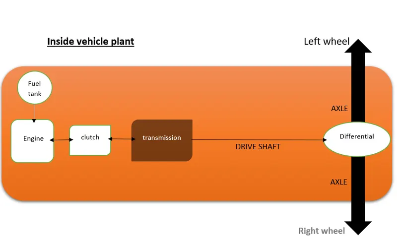
The powertrain is the usefuel linkages and the mechanical parts that combine together to transmit the power cranked put by the engine to the wheels. During power stroke, engine produces power which is transmitted to the clutch by the output shaft or crankshaft. The clutch on engaging with the transmission allows the power to travel to transmission. Here, according to the demand the power is regulated due to different gear ratios and then send to differential gear and finally to the wheels.
The power demand should have no lag during transmission. The time between the pressing of the throttle pedal and wheel rotation should have almost no lag in between. The input is in the form of acceleration, braking.
Efficiency - The fuel is consumed the moment the engine is turned on. The amount of fuel consumed is called fuel consumption and the fuel consumed to cover a distance is called efficiency.
The chemical energy is converted to heat energy so there is transfer of energy and mass from one system to another.
Mass flow rate is given by = (Engine power)/(transmission efficiency*engine efficiency*Qlhv)
The wheels when moving then it is called positive power and if the car is just idling or the clutch is disengaged then the power is considered as negative. The fuel is getting used even when it is idling to keep the engine to overcome the different pumping, friction losses in parts with surface contact.
There is another condition where the trottle is cut when the car is moving at such speed and the engine starts applying some braking force which cannot be avoided. The engine still consumes fuel to keep the engine in turned ON condition.
Fuel consumption depends on the power requirement at the wheels with no load or with some load, tire condition, road condition,driving style,engine condition etc.
There are different types of efficiencies :-
1)Mechanical efficiency - ratio of brake power and indicated power.
2)Indicated thermal efficiency - ratio of indicated power generated by the engine to the power generated by the combustion of the fuel.
3)Brake thermal efficiency - ratio of the brake power generated by the engine to the power generated by the combustion of the fuel.
4) Volumetric efficiency - ratio of the actual volume of the charge sucked into the cylinder at normal temperature and pressure to the volume swept by the piston in the cylinder.
Engine map
Engine mapping is also known as engine tuning in which the engine undergo some modification and adjustments at internal combustion engine and electronic control unit end. The mapping is done in order to increase the power output,efficiency etc.
Model
In map based model the predefined values of torque, air fuel mixture to give a relation between input and output, output and losses etc. The input given to the IC engine gives out the output. So, map is set in this IC engine end to give out a desired output.
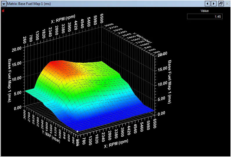
In analytical based model the input is given in terms of equation that defines the internal dynamics. The IC engine is studied by some computer software for thermal,design and matter flow.
There are two types of energy based models-
*)Forward model - The model that simulate from the input to the engine and all the way to the output i.e. the wheels. In general, it simulates the source to sink to determine the performance.
*)Backward model - The model simulates in the reverse order when compared to the forward model. It simulates the sink to source. Here, the output is the initial step where the vehicle speed and acceleration is taked ad input. These are then used to calculate the engine input which is the final output.
--This problem has a forward model.
1) Load the Project1 folder as the Current Folder in Matlab.(Completed)
2) Run the “Project1_InitFile.m” Matlab script.(Completed)
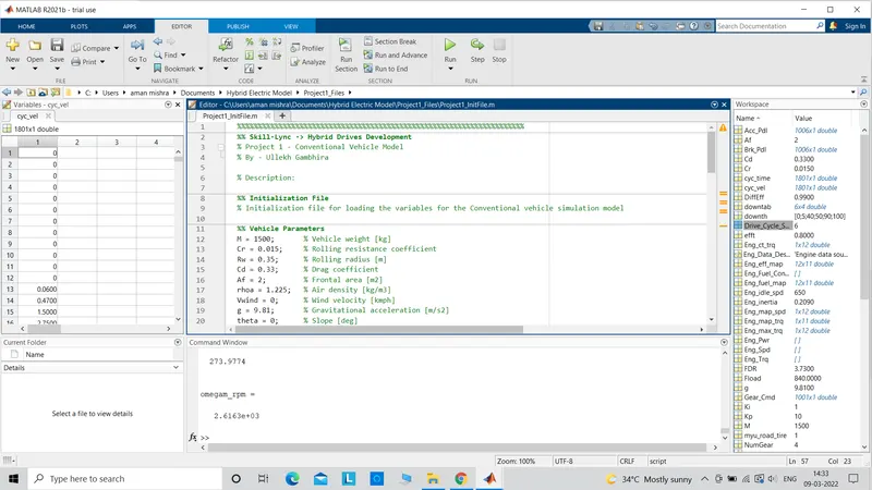
To begin the project, first I have downloaded the project from the portal and then ran the file in 'Matlab'. The following code gets uploaded.After runnung the code, I got all the defined variables with all the different cycles graphs. The program is nested with elseif function command. The function is set from 1-6 which represents the different cycles. The following graphs are obtained with corresponding cycles.
%%%%%%%%%%%%%%%%%%%%%%%%%%%%%%%%%%%%%%%%%%%%%%%%%%%%%%%%%%%%%%%%%%%%%
%% Skill-Lync -> Hybrid Drives Development
% Project 1 - Conventional Vehicle Model
% By - Ullekh Gambhira

% Description:

%% Initialization File
% Initialization file for loading the variables for the Conventional vehicle simulation model

%% Vehicle Parameters
M = 1500;       % Vehicle weight [kg]
Cr = 0.015;     % Rolling resistance coefficient
Rw = 0.35;      % Rolling radius [m]
Cd = 0.33;      % Drag coefficient
Af = 2;         % Frontal area [m2]
rhoa = 1.225;   % Air density [kg/m3]
Vwind = 0;      % Wind velocity [kmph]
g = 9.81;       % Gravitational acceleration [m/s2]
theta = 0;      % Slope [deg]
myu_road_tire = 1; % Coefficient of friction between tire - road interface
Tm=150; %motor torque
efft=0.8; %transmission efficiency
ratio=2.45; %Total ratio

%% Vehicle top speed
Vveh=sqrt((efft*ratio/Rw*Tm-Cr*M*g)*2/rhoa/Af/Cd) % Vehicle Velocity(m/s)
Vveh_kmph=Vveh*18/5 %Vehicle  velocity (kmph)

%% Power for Top speed
Fload=1/2*rhoa*Cd*Af*(Vveh+Vwind)^2+Cr*M*g*cosd(theta)+M*g*sind(theta) %Road load [N]
Pload=Fload*Vveh/1000 %Road load power [KW]

%% Powertrain Speed
omegam=ratio*Vveh/Rw  % motor speed in rad/s
omegam_rpm=omegam*30/pi % motor speed in rpm

%% Powertrain Parameters
FDR = 3.73;                         % Final Drive Ratio / Diff Ratio
DiffEff = 0.99;                     % Differential efficiency (assumed independent of operating conditions)

NumGear = 4;                        % Number of gears in transmission
TransGear = [1:NumGear];            % Transmission Gears
TransRatio = [3.06, 1.62, 1, 0.7];  % Corresponding Transmission ratios
TransEff = 0.90;                    % Transmission efficiency (assumed independent of operating conditions)

TC_SR = [0, .5, .6, .7, .8, .87, .92, .94, .96, .97, 1];   % Torque Converter Speed Ratio (Matlab default) -> TurbSpd/PumpSpd
TC_TR = [2.232, 1.5462, 1.4058, 1.2746, 1.1528, 1.0732, 1.0192, 1, 1, 1, 1];   % Torque Converter Torque Ratio (Matlab default) -> TurbTrq/PumpTrq
TC_Cf = 1e-4 * [.72558, .66322, .63463, .59042, .51331, .4144, .29287, .22444, .12186, .04386, 0]; % Torque Converter Capacity Factor (Matlab default) -> PumpTrq/PumpSpd^2 [Nm/rpm^2]

load Vehicle_Data/Engine_data_1_9L_Saturn_95kW
load Vehicle_Data/Trans_Shift_map

%% Driver Parameters
Kp = 10;                    % P gain for driver PI model
Ki = 1;                     % I gain for driver PI model
Drive_Cycle_Select =6;     % Drive cycle selection

% Drive cycle values in m/s

if Drive_Cycle_Select == 1
    load DriveCycles/UDDS;

elseif Drive_Cycle_Select == 2
    load DriveCycles/HWFET;

elseif Drive_Cycle_Select == 3
    load DriveCycles/FTP;

elseif Drive_Cycle_Select == 4
    load DriveCycles/US06;

elseif Drive_Cycle_Select == 5
    load DriveCycles/NEDC;

elseif Drive_Cycle_Select == 6
    load DriveCycles/WLTP;

end

time_end = cyc_time(end);
vel_end = cyc_vel(end);

figure(10)
plot(cyc_time,cyc_vel,'linewidth',3,'color','b')
xlabel('time')
ylabel('Vehicle speed')
grid on
3)Model
Vehicle dynamics (Completed)
Engine (Completed)
6)Report is as follows:-
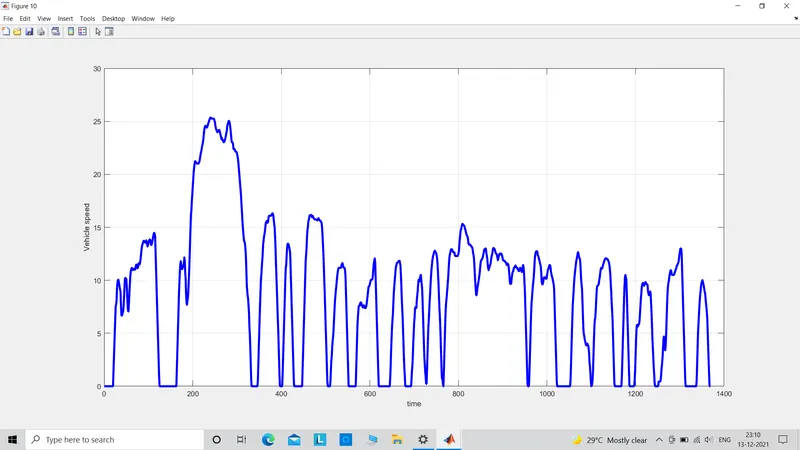
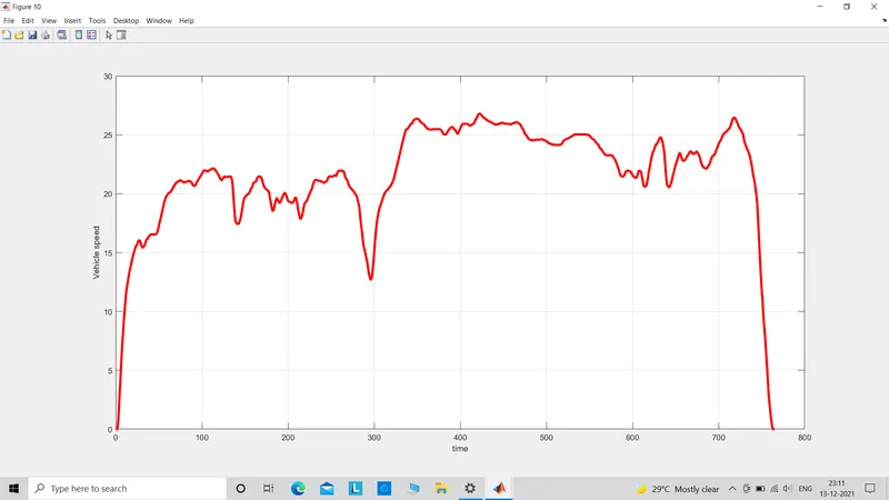
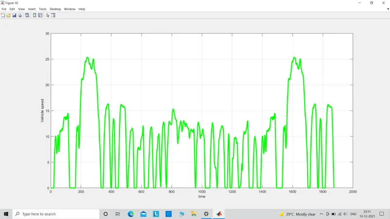
After running the above code, the following drive cycles are obtained as a result.
The cycle uploaded are:-
*)Urban Dynamometer Driving Schedule or UDDS:-
*)Highway Fuel Economy Test cycle or HWFET:-
*)Federal Test Procedure or FTP:-
*)Supplemental Federal Test Procedure or US06:-
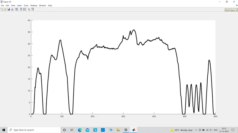
*)New European Driving Cycle or NEDC:-
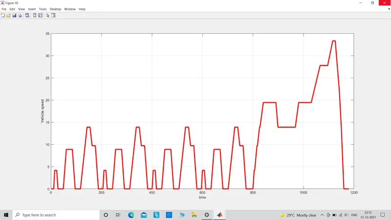
*)Worldwide harmonized Light vehicles Test Cycles or WHLVTC:-
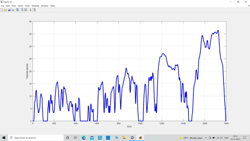
The only two cycles used in this project are UDDS and HWFET drive cycle.
The Simulink Model {UDDS) :-
Driver block
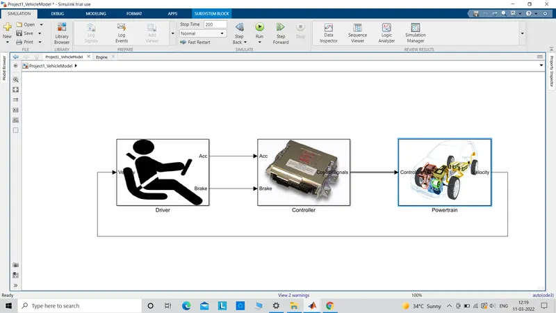
The vehicle model project consists of basic three blocks which are Driver,Controller and Powertrain and it is clearly visible that it is a forward energy based model. It is formed in a loop. The input of driver block is the velocity and time. Time is taken independently to simulate the driver block whereas the velocity is the feedback that comes from the vehicle dynamic block inside powertain block. The output of the driver block is how much the accelerator and brake pedal is pressed or released.
Inside Driver block
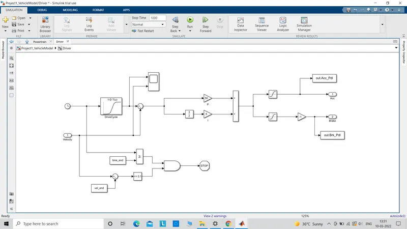
The graph
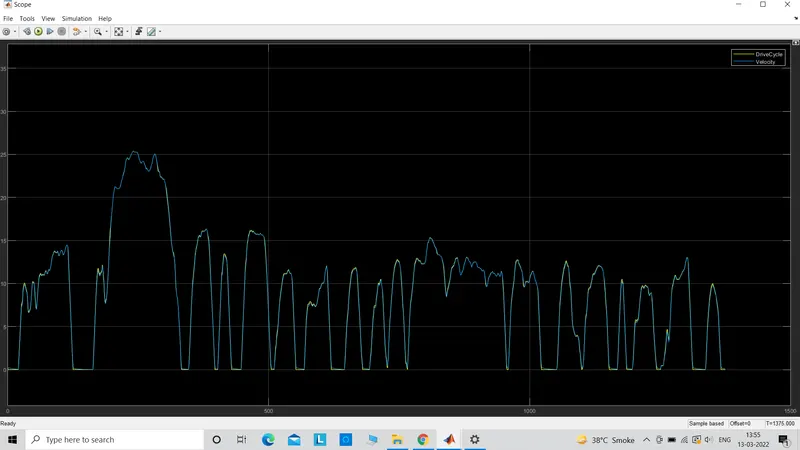
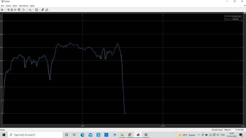
The above graph is between time, drive cycle and velocity. So the predetermined set of values with speed and distance give out the ideal UDDS cycle graph and the velocity values fed independdently is triying to trace the same curve as the former one.
Controller block
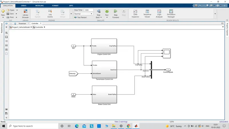
This is a processing block so computer controlled unit is introduced here ECU. Engine control unit collects the speed of the engine, vehicle and more to give out a desired performance. It has a ideal engine speed controller which makes sure that the speed of the engine does not go below a set value of the rpm. So whatever throttle input is given by the driver is getting converted to engine torque request.
Engine Control Unit
The block controls the engine stays in the range predefined and the engine speed does not cross the highest value set in the table provided.
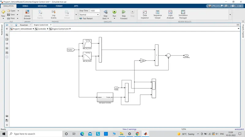
The graph associated with the above block for UDDS cycle
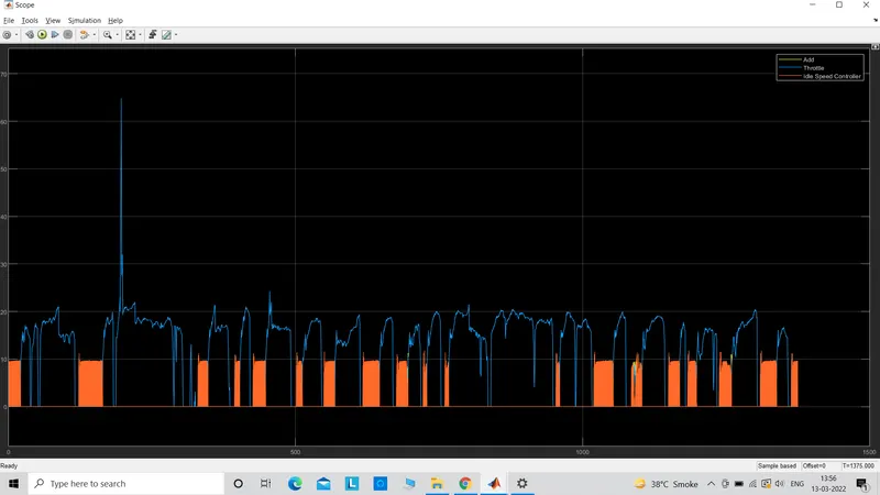
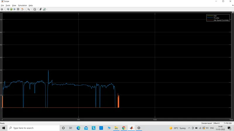
The graph shows the input speed given to it and the work done by the the electonic controller to keep the engine to the minimum rang when it idealing to aovid turning off of the engine when the car is in neutral.
Ideal Speed controller
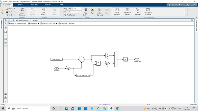
It keeps the engine in the ideal runnung state which means when the engine is ignited, the ideal speed controller makes the engine to maintain a constant low rpm until the throttle is pressed.
Transmission control unit
Second is the transmission control unit(TCU) which is a electronically controlled gear box control system, collects the data and ensures that the gear shifting is smooth without any hinderance. This block takes throttle and vehicle speed as input and then there is a shift logic that has been preset to speed range for each gear. So depending on the input, the gear will change and give the gear command as output.
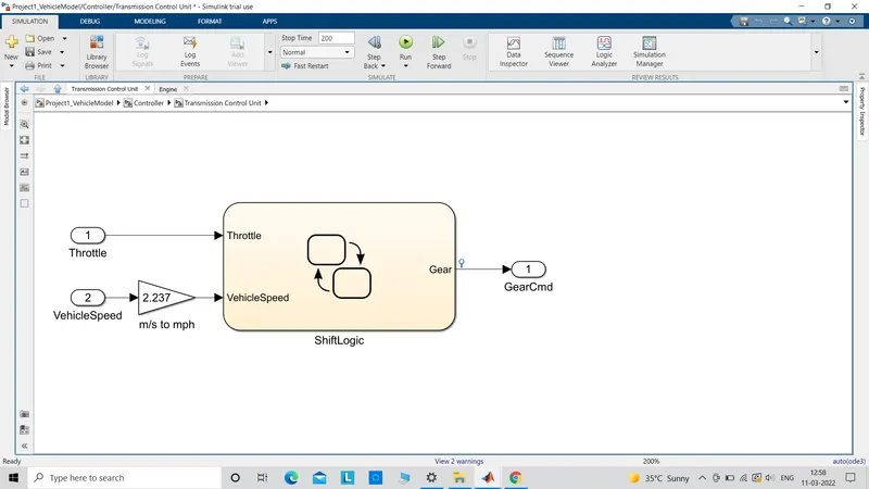
Brake control unit
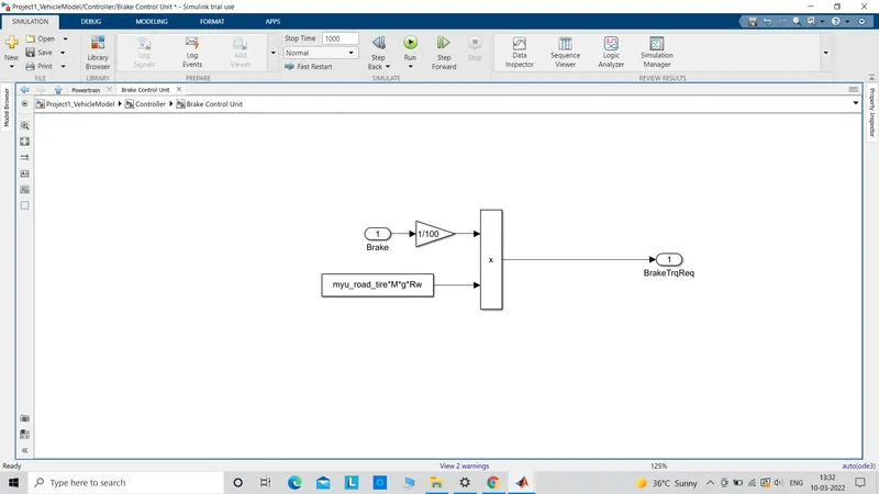
Third is the brake control unit which takes in the data as per the degree of pedal pressed or released. The brake input is accompanied by the other forces at on the car which acts as a resistance and together these all give output as the brake request.
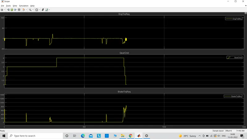
Together the three different outputs are engine torque request, gear command,brake torque request.
The graph
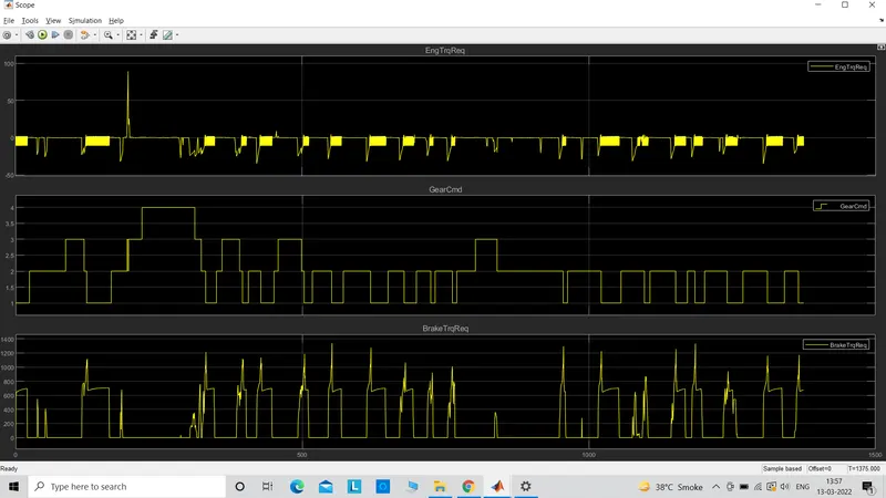
The above graph shows the torque requirement which could be accelerating the car known as positive torque or negative torque used at the time when the car is braked by the disc brake or engine braking. The next curve is the present gear number at that instant. The graph rises shows the gear is set to high while lowering of the graph shows the speed is reducing and the engine is down shifted to a lower gear. The last one is the brake torque which is experienced at the time of wheel braking or engine braking. The three graph show how each other behave when any of the three is changed in terms of values.
The controller signals are fed into the powetrain block. Powertrain is a network of cables and linkages which connects the major different mechanical components so that the power cranked out of the engine could be transferred uniterruptedly from the engine to the wheels.
Inside the powertrain block
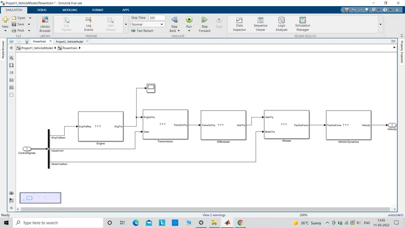
There are engine, transmission, differential,wheels and vehicle body blocks all connected as shown above. The engine block is fed with the engine torque signals from the controller. Gear command signals are fed into the transmission and brake torque signals are fed into the wheels.
Engine block
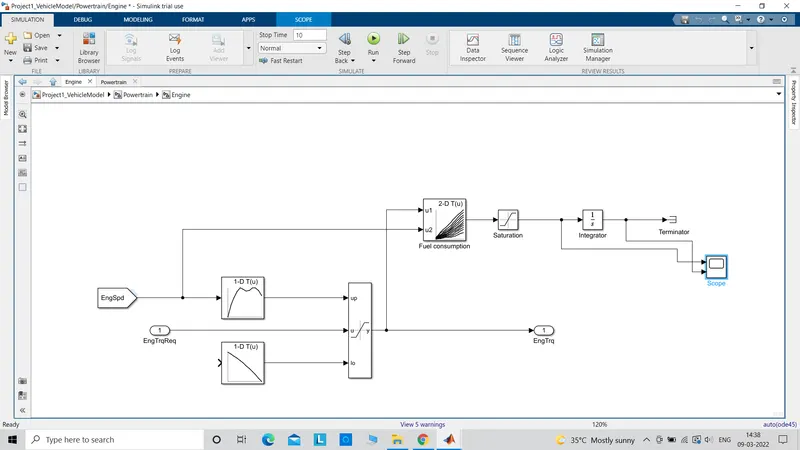
The engine block uses the engine torque request signals and check if the torque is in between the predefined range provided by the map. Same goes for the speed where speed values are sent and processed by the map i.e. the UDDS map and then the fuel consumption and fuel flow rate can be obtained.
The graph
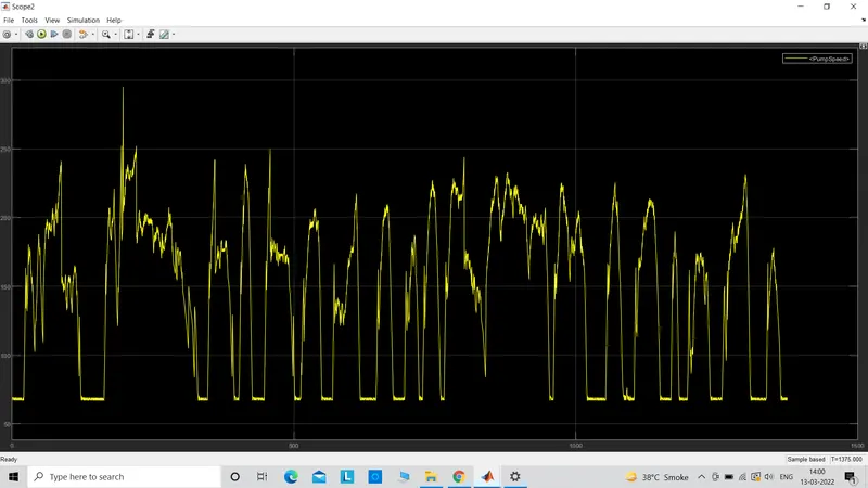
The below graph shows the variation in the engine input speed given to the engine by the controller according to the driver block.
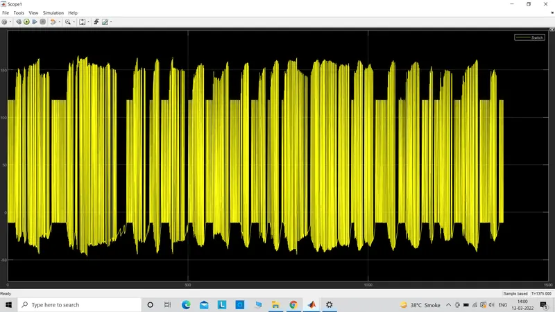
The below graph is the torque produced or output torque in result of the input engine speed given to the engine block as explained earlier.
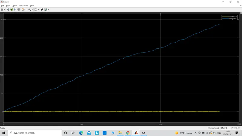
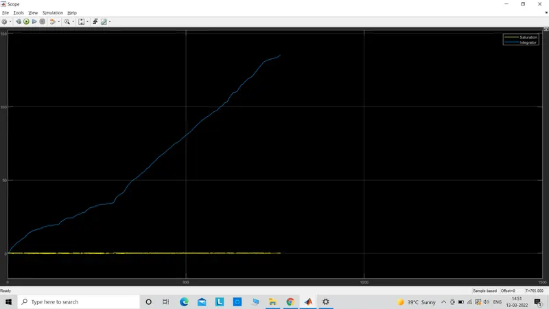
The above graph shows the yellow curve which is nearly linear is the rate of the fuel getting used up by the engine in order to produce that torque output to move the car. The blue curve is nearly rising at a constant rate which represents the fuel consumption. So on integrating the fuel rate, we get fuel consumption. As the fuel rate is increasing, the consumption is increasing as well.
Transmission block
The output engine torque is fed into the transmission block along with the gear command signals.
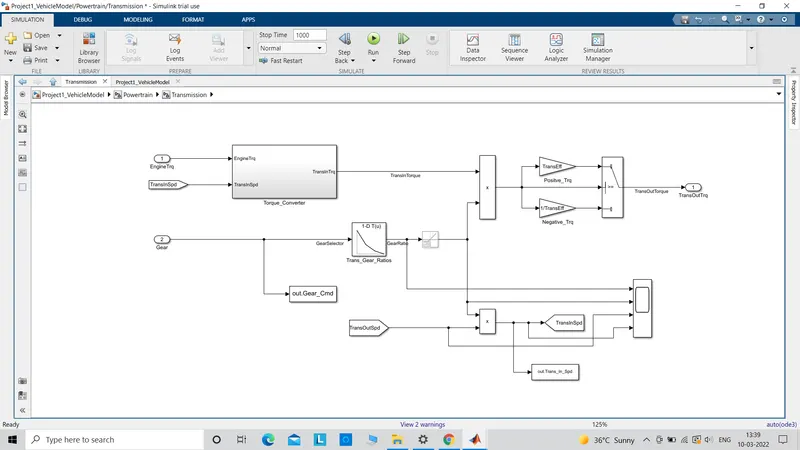
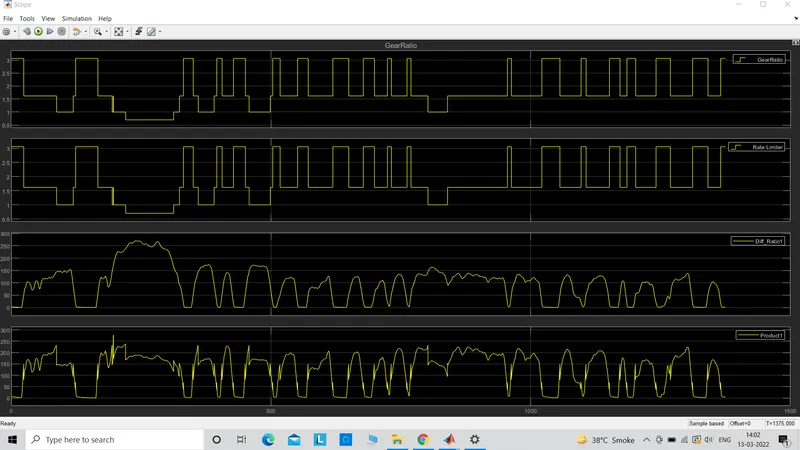
The above graph for UDDS drive cycle traces a curve according to the input drice cycle. So in order to run the car accordingly, the above gear demand and torque which become the input. The output transmission torque is traced after going through the different gear ratios.
The transmission in this case has a torque converter which sets the speed of the car depending on the torque input.
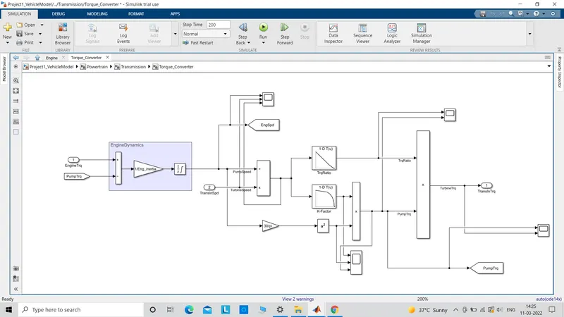
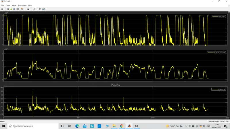
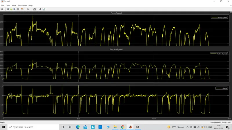
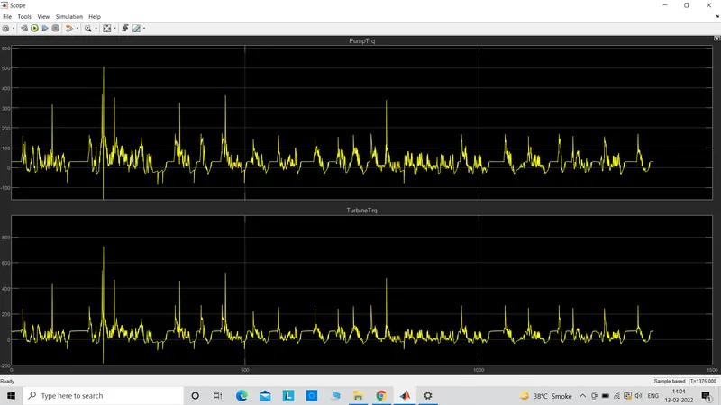
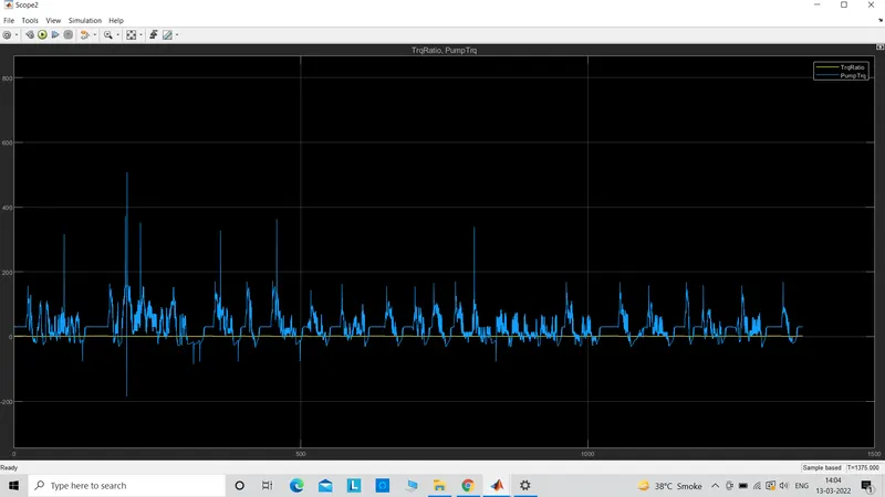
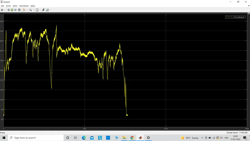
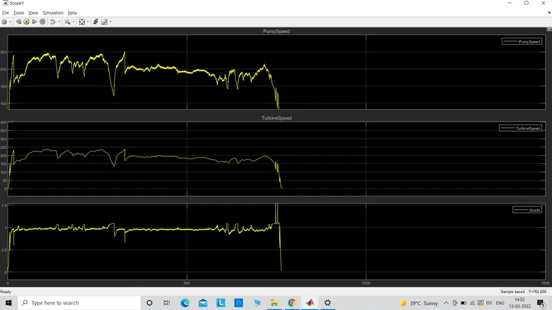
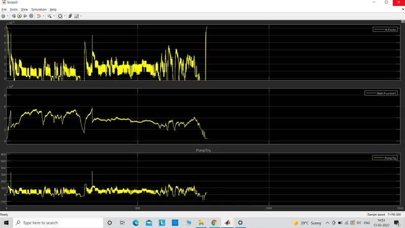
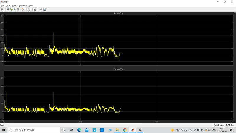
The above graphs states the input and output of the torque convertor getting used in this case. The turbine and the pump speeds. The pump when rotates forces the fluid to move the turbine and the torque produced by both is traced above.
Differential block
The transmission output torque is then fed to the differential block.
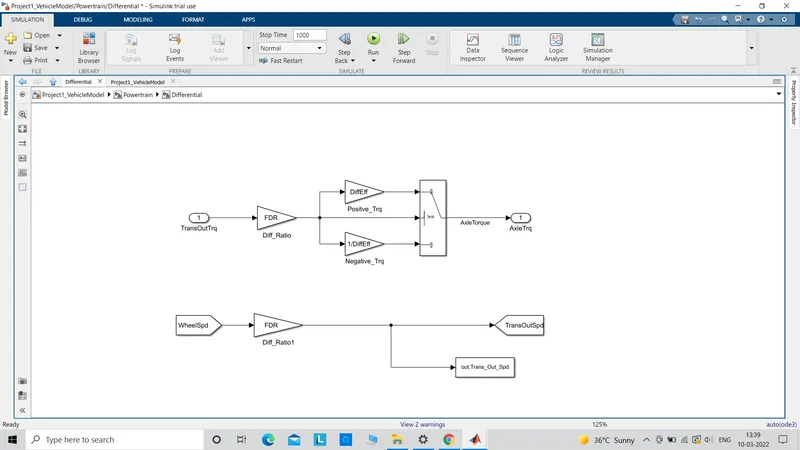
The transmission torque goes through the condition where the torque is positive or negative and the output becomes the axle torque which is obviously at lower than the transmission torque due to friction losses. The wheel speed is fed into the differential gear ratio as it has a planetary gear system and the transmission output speed is obtained as an output which is thr transmission rpm.
Wheels block
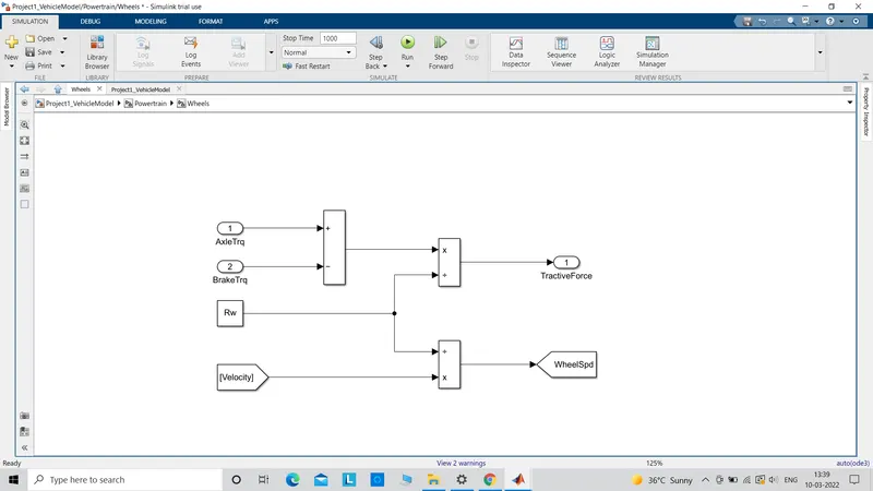
The power and torque obtained out of the differential is then fed to the wheels with transmission output rpm and wheel speed as input to Wheel block. So this in turn will move the wheels according to the input power and torque. If the torque is negative than the wheel is actually stopping. The output is the tractive force that the wheel develops as it comes into motion and also the speed of the wheel.
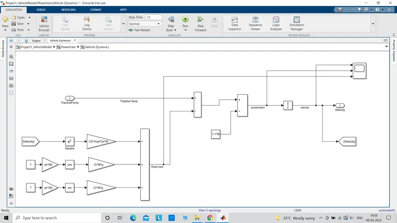
Vehicle dynamic block
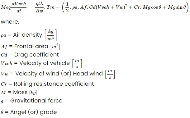
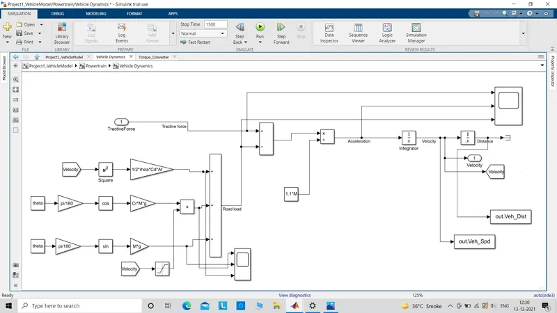
Vehicle dynamic block is the where the whole body and wheel feel the forces when it is moving. The tractive force is the input along with aerodynamic drag,rolling force adn weight of the body. According to the equation, the block is designed. The output is the velocity the car acheived which is back looped with the drive block for feedback and to continue the cycle for the desired vehicle performance output.
The graph
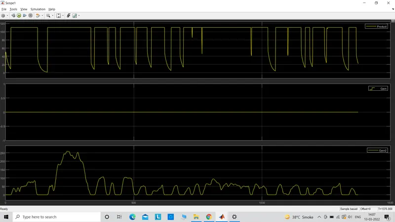
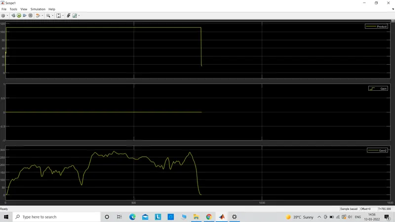
This graph shows the forces like aerodynamic drag,rolling friction and the weight of the body values as input to the body dynamic in form of curves.
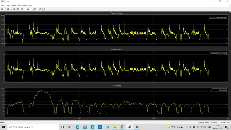
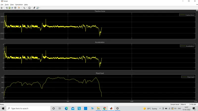
The below curve shows the output of the tractive force,acceleration and roadload as input again to the car, The acceleration reduces as the tractive and road load increases which brings in the above mentioned forces to stop the vehicle. So, greater the speed of the car, greater the forces trying to stop the car.
Simulink model graphs for HWFET
To load the HFWET values, just type 2 in the matlab code select the drive cycle
The same blocks are used in this drive cycle also, it is just that when the matlab code is run the HWFET cycle gets loaded in the matlab and simulink everywhere where UDDS was loaded earlier.
The graph
Driver block.
Engine block.
ECU
Engine block.
Transmission block.
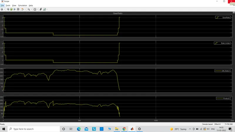
Torque converter.
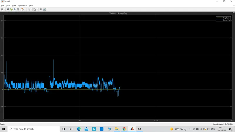
Vehicle dynamics.
3) The provided vehicle Simulink model “Project1_VehicleModel.slx” is incomplete. The engine and vehicle dynamics block contents have been deleted. Build the Simulink blocks by referring to the course lecture and example block images provided. You can run the model and analyze the results using a ‘Scope’ for debugging.(Completed)
4) Add additional ‘To Workspace’ blocks for transferring the desired Simulink vehicle data into the Matlab workspace.(Completed)
5) Modify the “Project1_ProcessingFile.m” as per the desired plots and required calculations.(Completed)
Post modeling plotting code
The code actually had all the varialbles which would load in the workspace after the code is run. But to get all the values I had to attach the to workspace block to import all the result values to the matlab workspace. This helped to get all the array of the values that was used later to plot the graphs.
There I had to change the 'goto' velocity block settings from local to global so that the block's value gets used up everywhere in the model.
The model picture could be used by going to mask options and select which image you want to use. This helps in recognizing the block easily.
Matlab Plots
For UDDS
1)Fuel consumption vs flow rate
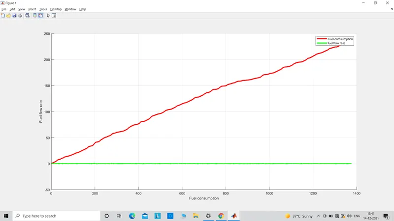
The UDDS drive cycle has a rising fuel rate with fuel consumption curve. It is quite obvious that if the fuel flow rate is constant then the fuel consumption is almost constant if I neglect the engine temperature losses and other losses. The fuel flow rate increases as the accelerator pedal is wide open increasing the fuel consumption. This also reduces the fuel economy. In this cycle the car is moving in city condition where it has to accelerate then brake and the cycle repeats irregularly. This means that the engine has to pull the car from rest all the time which increases the fuel requirement by the engine to bring th heavy overal mass of the car to motion and once it is in motion it requires less fuel. In city, the car is never moving at a constant speed but accelerating and braking and while acceleration as explained earlier, the fuel consumption increases. One more reason is the cold temperature of the engine because the car has to make short trips which means the engine does not reach a warm transient temperature at which the engine runs better. More fuel is used to keep a cold engine running than a warm engine. Then the distance travelled in a certain amount of fuel consumed is also less because when the car encounters traffic signal with red light, the car stops with mostly the engine on making the car go nowhere even when the fuel is consumed. This again is treated as high consumption during the cycle.
2)Plot the time trace for engine, transmission input, transmission output and wheel speed on one plot
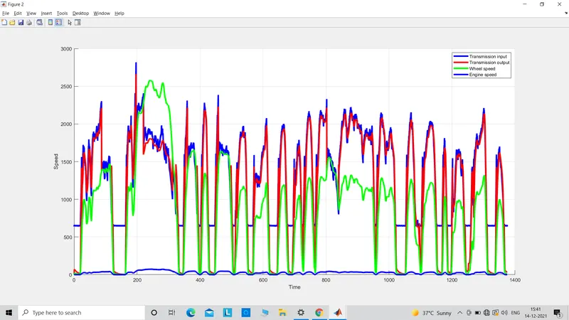
The graph shows that the transmission output and input speed are not getting traced identical. This means the torque converter which is used to achieve the diffferent gear ratios have some losses in between the turbine and the impeller. This shows that the impeller shaft moves at comparetively higher rpm thant he turbine shaft as they are not connected directly but oil makes them to rotate. The graph also shows the engine and wheel speed variation in the speed over the entire cycle. Due to the transmission the engine rotates at different speed but the change in wheel speed is constant. The engine would touch 9000rpm many times at different gears but the car wheel would reach the top speed only at the top most gear. The bottom curve shows the wheel speed of the car following this cycle.
3) Plot engine torque, engine power, fuel rate and fuel consumption using subplots
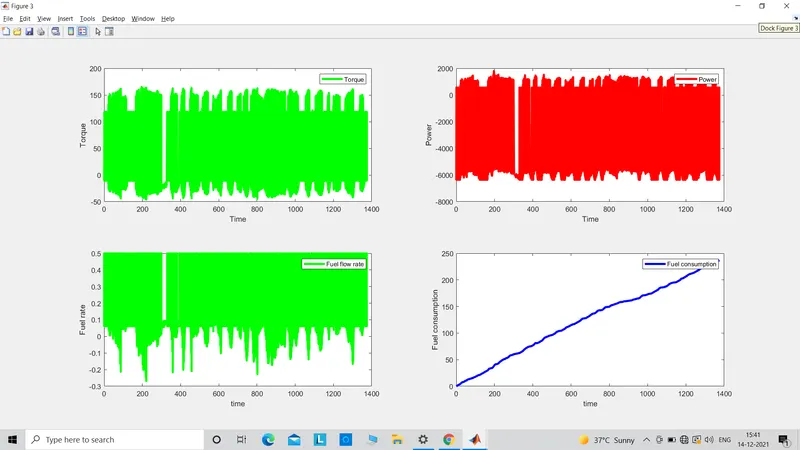
i) The graph is between time (sec) and torque (Nm). The torque requirement shows a huge variation on the entire time range. This is due to make the car move from all the stops and accelerate in city condition. At the braking time the torque is used to stop the car which is negative. So more aggressive plummeting is observed due to hard braking due the city conditions.
ii) The power is lost more than it is used to drive the car. This is again due to the city conditions. Power is dependent on torque and power comes into picture when the car starts moving at an average or above average speed. Basically, power helps to achieve a better top speed but in city, top speed can't be reached so torque is more important than power over here.
iii)The graph shows the variation of fuel rate with fuel consumption which is quite obvious. This is the reason why mileage is not good in city condition compared with HWFET drive cycle.
iv) The graph shows the fuel consumed over a period of time in city condition. It is rising till around 800. Then there is small drop in the consumption and then the curve rises with a lesser consumed rate.
4) Plot accelerator and brake pedal, gear command, vehicle desired and actual speed, vehicle distance using subplots
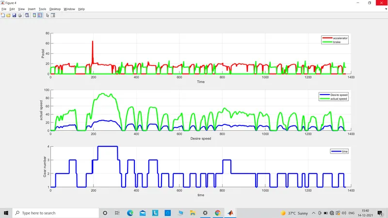
i) The graph is between acceleration pedal and brake pedal. So whenever the accelerator is pressed, the brake pedal is left untouched. So goes the other way round in which when the brake is pressed, acclerator is not used. However some regions on the graph is observed with situations where the accelerator is pressed a bit with brake this is at the time of bringing the car in motion from ideal state. This is done however to avoid the car from rolling in reverse direction due to its mass. The graph is for UDDS cycle so whereever in the cycle there is rise in speed, the accelerator is pressed and where the speed is reduced that means the car is braked.
ii) The graph is between the actual and desired speed vs time and it is clear that both the graph follow the same pattern. The only different is that the desired speed works in the lower region(rpm) in the graph whereas the actual speed is working in the upper region rpms in the graph.
iii) The graph shows the gear position in following the UDDS cycle. So the graph traces the same city cycle. Whenever the speed in increasing, the engine is upshifted to higher gear. Whenever the car is braked, the engine is downshifted to lower gear. The transmission is 4 speed automatic one. Almost all the time the car is changing the gears from low to high and vice versa and also it remains at 2nd gear most of the time.
All the three graphs are linked together and states that when the accelerator pedal is pressed, the engine will increase the rpm which in turn will make the car to increase the speed. this will make the car to upshift gears according to the speed. The same logic is followed at the time of braking.
5) Plot the engine operating points on the engine fuel map
The fuel is actually the summery of the engine operating in the entire operating regime from dead idling to full load at full throttle and every possible condition in between.
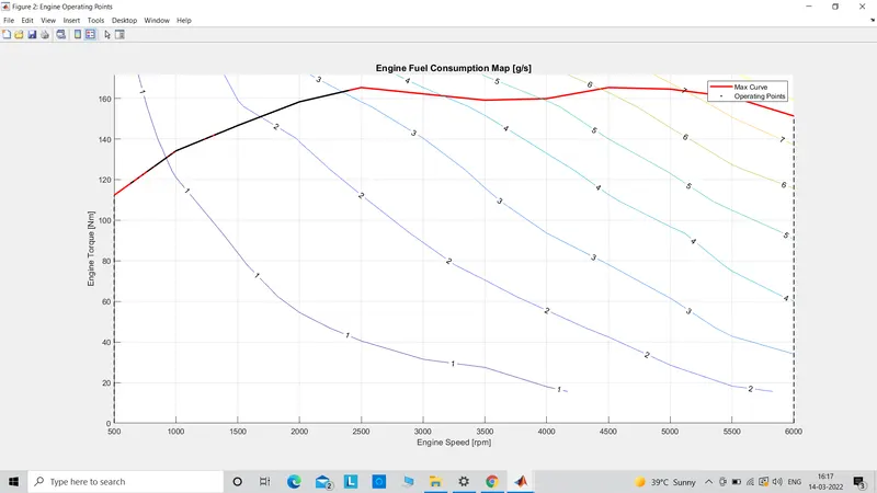
On x-axis, we have the engine speed in rpm with engine torque in Nm on y-axis. Often torque is replaced by brake mean effective pressure term. The chart is used to test different cars in different load conditions. The red curve that is visible on the graph is the peak torque curve with respect to time. Here, the car has a 1.9 litre engine with 4-speed automatic transmission. So the torque actually is rising till 2500 rpm then it dorps a bit and maintains the curve till 6000 rpm. with the peak at around 2500 and 4500 rpm for this cycle. That peak value gives the highest torque produced by the car at that rpm. The engine if further stretched to higher rpm will blow the engine right away. Where there is a circle in a region on this graph, that is called bull's eye which also makes this map to be known as bull's eye map. The curves at the outer portion means more consumption of the fuel with the inner curves indicating less fuel consumption. Fuel consumption increases in conditions like high load at idling and low load at high rpm. Fuel consumption is more likely to give the efficiency which increases when the engine is operating at moderate load and at mid rpms.
For HWFET
1)Fuel consumption vs flow rate
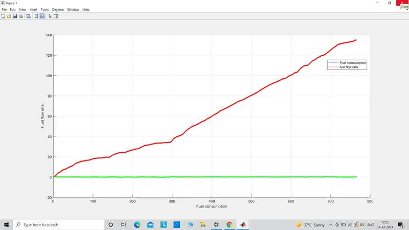
The HNFET drive cycle has a lazy rise in fuel rate with fuel consumption curve over time. It is quite obvious that if the fuel flow rate is constant then the fuel consumption is almost constant if I neglect the engine temperature losses and other losses. The fuel flow rate increases as the accelerator pedal is wide open increasing the fuel consumption. This also reduces the fuel economy. In this cycle the car is moving in highway condition where it almosts cruises at a constant speed with low use of brake and also at constant pressed accelerator position. This means that the engine once after coming in motion has no linger going to pull the car hard. This means that it has to accelerate only once when it starts to move from rest and till the time it reaches the desired speed. The car is then made to run at that constant small bandwidth speed range which exerts less pressure on the engine because the car is no longer pulling its mass as hard as it was doing at the time it came in motion or when it was accelerated. On highways, the car is moving at a constant speed and the fuel consumption is reduced. One more reason is the cold temperature of the engine because the car has already reached the warm operating temperature, the engine no longer is stressed to work. More fuel is used to keep a cold engine running than a warm engine. Then the distance travelled in a certain amount of fuel consumed is also less because when the car does not encounter traffic signal often. The the car does not stop much and the fuel is used less and the car travels a much longer distance. The cycle is efficient only when the car is not made to touch the top speed because then all the aero drag, rolling friction and weight which are diretly proporional will imporve with square of the velocity.
2) Plot the time trace for engine, transmission input, transmission output and wheel speed on one plot
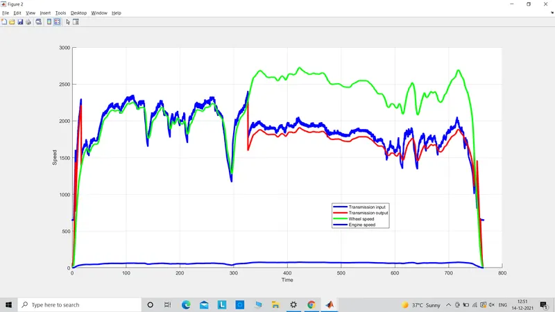
The graph shows that the transmission output and input speed are not getting traced identical. This means the torque converter which is used to achieve the diffferent gear ratios have some losses in between the turbine and the impeller. This shows that the impeller shaft moves at comparetively higher rpm thant he turbine shaft as they are not connected directly but oil makes them to rotate. The graph also shows the engine and wheel speed variation in the speed over the entire cycle. Due to the transmission the engine rotates at different speed but the change in wheel speed is constant. The engine would touch 9000rpm many times at different gears but the car wheel would reach the top speed only at the top most gear. The bottom curve shows the wheel speed of the car following this cycle.
3) Plot engine torque, engine power, fuel rate and fuel consumption using subplots
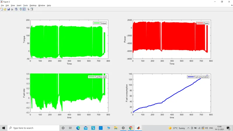
i) The graph is between time (sec) and torque (Nm). The torque requirement shows less variation on the entire time range. This is due to make the car move at almost constant speed on highway and it remains at the torque region because no high values of torque is required for an already in motion car. At the braking time the torque is used to stop the car which is negative. So almost a smooth graph is observed.
ii) The power is used in this cycle because the car is operating at higher speed range. This is again due to the highway condition. Power is dependent on torque and power comes into picture when the car starts moving at an average or above average speed. Basically, power helps to achieve a better top speed but in city, top speed can't be reached so torque is less used than power over here.
iii)The graph shows less variation of fuel rate with fuel consumption which is quite obvious. This is the reason why mileage is good in highway condition compared with UDDS drive cycle.
iv) The graph shows the fuel consumed over a period of time in city condition. It is lazy till 300. Then there is small drop in the consumption and then the curve rises with a constant rate and it is clear the comsumption is less in this cycle.
4) Plot accelerator and brake pedal, gear command, vehicle desired and actual speed, vehicle distance using subplots
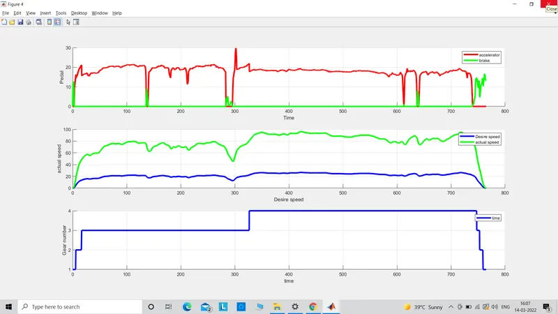
i) The graph is between acceleration pedal and brake pedal. So whenever the accelerator is pressed, the brake pedal is left untouched. So goes the other way round in which when the brake is pressed, acclerator is not used. However some regions on the graph is observed with situations where the accelerator is pressed a bit with brake this is at the time of bringing the car in motion from ideal state. This is done however to avoid the car from rolling in reverse direction due to its mass. The graph is for HWFET cycle so whereever in the cycle there is rise in speed, the accelerator is pressed and where the speed is reduced that means the car is braked.
ii) The graph is between the actual and desired speed vs time and it is clear that both the graph follow the same pattern. The only different is that the desired speed works in the lower region(rpm) in the graph whereas the actual speed is working in the upper region rpms in the graph.
iii) The graph shows the gear position in following the HWFET cycle. So the graph traces the same high speed highway cycle. Whenever the speed in increasing, the engine is upshifted to higher gear. Whenever the car is braked, the engine is downshifted to lower gear. The transmission is 4 speed automatic one. The car remains in the top gear 4th gear for the maximum time which shows the car is moving at a constant high speed range.
All the three graphs are linked together and states that when the accelerator pedal is pressed, the engine will increase the rpm which in turn will make the car to increase the speed. this will make the car to upshift gears according to the speed. The same logic is followed at the time of braking.
5) Plot the engine operating points on the engine fuel map
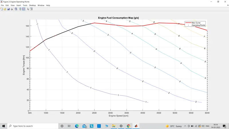
On x-axis, we have the engine speed in rpm with engine torque in Nm on y-axis. Often torque is replaced by brake mean effective pressure term. The chart is used to test different cars in different load conditions. The red curve that is visible on the graph is the peak torque curve with respect to time. Here, the car has a 1.9 litre engine with 4-speed automatic transmission. So the torque actually is rising till 2500 rpm then it dorps a bit and maintains the curve till 6000 rpm. with the peak at around 2500 and 4500 rpm for this cycle. That peak value gives the highest torque produced by the car at that rpm. The engine if further stretched to higher rpm will blow the engine right away. Where there is a circle in a region on this graph, that is called bull's eye which also makes this map to be known as bull's eye map. The curves at the outer portion means more consumption of the fuel with the inner curves indicating less fuel consumption. Fuel consumption increases in conditions like high load at idling and low load at high rpm. Fuel consumption is more likely to give the efficiency which increases when the engine is operating at moderate load and at mid rpms.