Project 1
TITLE : DEVELOPMENT OF A FORWARD ENERGY BASED FUEL CONSUMPTION MODEL OF A CONVENTIONAL VEHICLE
AIM
- Writing scripts in MATLAB and load the variables required for running simulink model
- Build simulink model using blocks and complete the model
- Plot Engine Torque , Power , Fuel Rate , Fuel Consumption using subplots.
- Plot time for Engine ,Transmission IN/OUT put
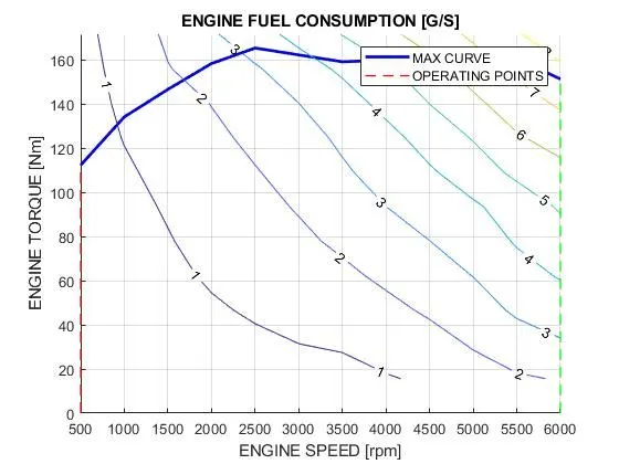
- Plot Engine Operating Points on Engine Fuel Map
- Plot Accelerator , Brake , Gear , Vehicle desired and Actual speed Vehicle distance using subplots.
- Tabulate the fuel economy for USSD AND HWFET Cycle.
- Generate plots for both Cycle.
THEORY
Conventional vehicle internal combustion engine fueled by gasoline or diesel to power the wheels .
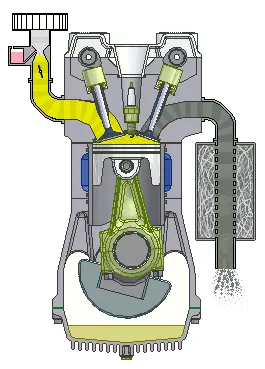
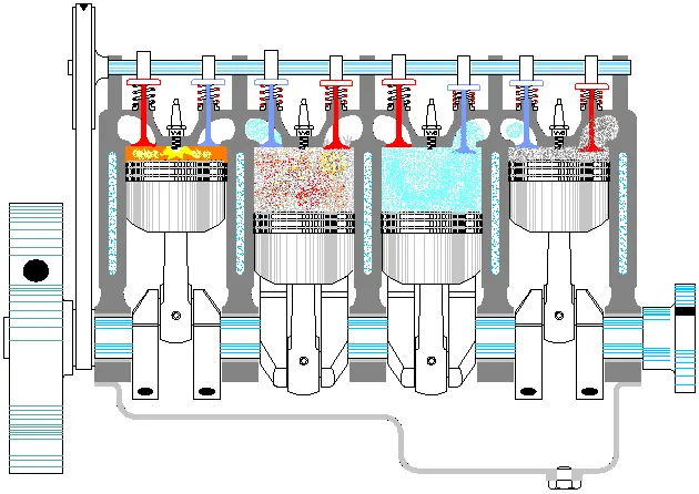
A petrol engine or gasoline engine is an internal combustion engine with the spark ignition designed to run on the petrol and similar volatile fuels . In most petrol engine the fuel and aur are usually premixed before compression . An internal combustion engine having its piston driven by the explosions of a mixture of air and vaour of a gasoline or the volatile fuels ignited by an electric spark.
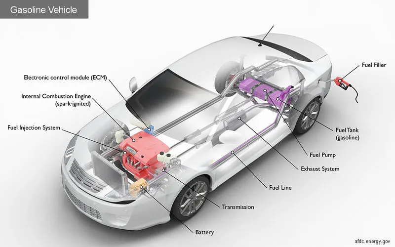
- Battery The Battery provides electricity to start engine and power vehicle electronics accessories.
- ECM The CM controls the fuel mixture ignition timing and emissions system monitors the operation of the vehicle safeguards the engine from abuse and detects and trouble shoots problems.
- Exhaust system The exhaust system channels the exhaust gases from the engine out through the tailppe . A three way catalyst is designed to reduce to reduce engine out emission within the exhaust system
- Fuel Filler A nozzle from a fuel dispenser attaches to the receptable on the vehicle to fillthe tank
- Fuel Injection system This system introduces fuel into the engine combustion chambers for ignition
- Fuel line A metal tube transfer fuel from the tank to the engine fuel injection system
- Fuel Pump A pump that transfers fuel from the tank to the engine fuel injection system via fuel line.
- Fuel Tank This tank stores gasoline on board the vehicle until its needed by the engine
- Internal Combustion engine In this fuel is injected into either the intake manifold or the combustion chamber where it is combined wit air fuel mixture is ignited by the spark from a spark plug.
- Transmission The transmission transfers mechanical power from the engine and or electric traction motor to drive the wheels.
CODE
%%%%%%%%%%%%%%%%%%%%%%%%%%%%%%%%%%%%%%%%%%%%%%%%%%%%%%%%%%%%%%%%%%%%%
%% Skill-Lync -> Hybrid Drives Development
% Project 1 - Conventional Vehicle Model
% By - VIKAS

% Description:

%% Initialization File
% Initialization file for loading the variables for the Conventional vehicle simulation model

%% Vehicle Parameters
M = 1500;       % Vehicle weight [kg]
Cr = 0.015;     % Rolling resistance coefficient
Rw = 0.35;      % Rolling radius [m]
Cd = 0.33;      % Drag coefficient
Af = 2;         % Frontal area [m2]
rhoa = 1.225;   % Air density [kg/m3]
Vwind = 0;      % Wind velocity [kmph]
g = 9.81;       % Gravitational acceleration [m/s2]
theta = 0;      % Slope [deg]
myu_road_tire = 1; % Coefficient of friction between tire - road interface

%% Powertrain Parameters
FDR = 3.73;                         % Final Drive Ratio / Diff Ratio
DiffEff = 0.99;                     % Differential efficiency (assumed independent of operating conditions)

NumGear = 4;                        % Number of gears in transmission
TransGear = [1:NumGear];            % Transmission Gears
TransRatio = [3.06, 1.62, 1, 0.7];  % Corresponding Transmission ratios
TransEff = 0.90;                    % Transmission efficiency (assumed independent of operating conditions)

TC_SR = [0, .5, .6, .7, .8, .87, .92, .94, .96, .97, 1];   % Torque Converter Speed Ratio (Matlab default) -> TurbSpd/PumpSpd
TC_TR = [2.232, 1.5462, 1.4058, 1.2746, 1.1528, 1.0732, 1.0192, 1, 1, 1, 1];   % Torque Converter Torque Ratio (Matlab default) -> TurbTrq/PumpTrq
TC_Cf = 1e-4 * [.72558, .66322, .63463, .59042, .51331, .4144, .29287, .22444, .12186, .04386, 0]; % Torque Converter Capacity Factor (Matlab default) -> PumpTrq/PumpSpd^2 [Nm/rpm^2]

load Vehicle_Data/Engine_data_1_9L_Saturn_95kW
load Vehicle_Data/Trans_Shift_map

%% Driver Parameters
Kp = 10;                    % P gain for driver PI model
Ki = 1;                     % I gain for driver PI model
Drive_Cycle_Select = 1;     % Drive cycle selection

% Drive cycle values in m/s

if Drive_Cycle_Select == 1
    load DriveCycles/UDDS;

elseif Drive_Cycle_Select == 2
    load DriveCycles/HWFET;

elseif Drive_Cycle_Select == 3
    load DriveCycles/FTP;

elseif Drive_Cycle_Select == 4
    load DriveCycles/US06;

elseif Drive_Cycle_Select == 5
    load DriveCycles/NEDC;

elseif Drive_Cycle_Select == 6
    load DriveCycles/WLTP;

end

time_end = cyc_time(end);
vel_end = cyc_vel(end);
In this project, a typical midsize car with a 1.9L engine and a 4-speed automatic transmission is considered. Data is taken from ADVISOR data base developed by NREL, USA. Transmission shift map and controller is taken from Matlab/Simulink example database. The model developed has the capability to simulate the vehicle on different drive cycles like UDDS, HWFET, FTP, NEDC, etc.
“Project1_InitFile.m” is a Matlab script used to load all the variables required for running the Simulink model and for post-processing. The drive cycle selection is also done here. Before running the Simulink vehicle model, run this initialization script.
SIMULINK MODEL
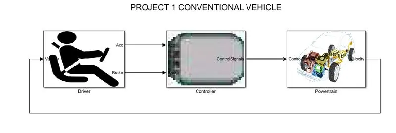
DRIVER
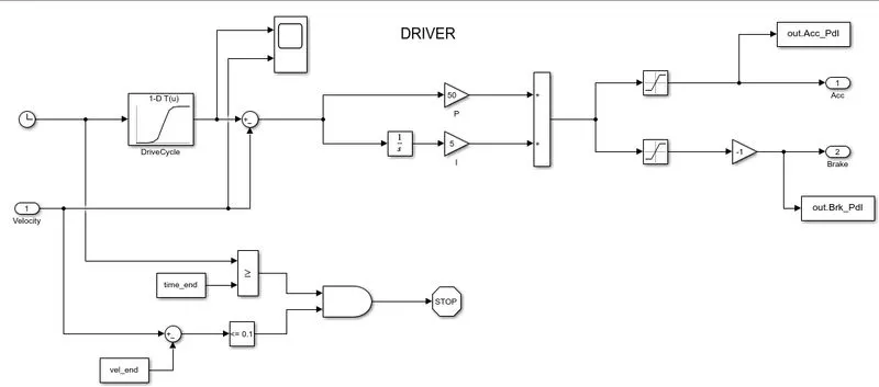
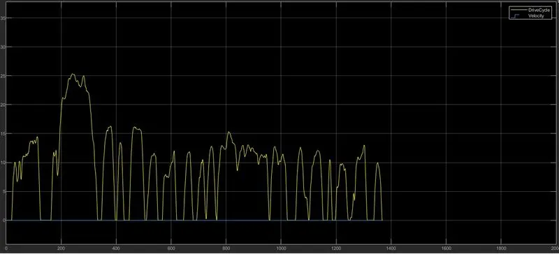
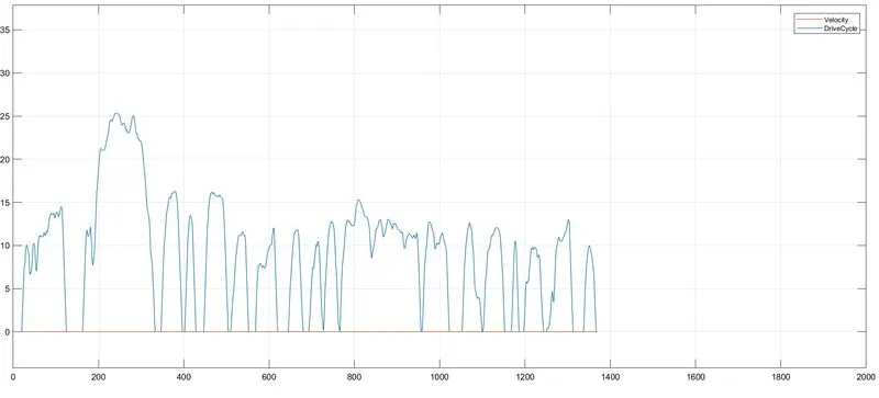
Driver block is a basic PI controlle r that genertaes acclerator and brake pedal to match desired and actual vehicle speeds .It is based on time , velocity then it all integrate creates output accleration and brajke pedal
Graph Results
CONTROLLER
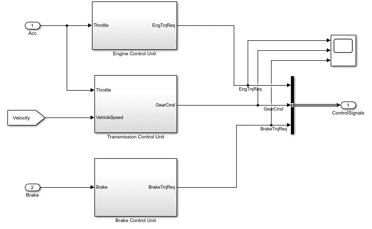
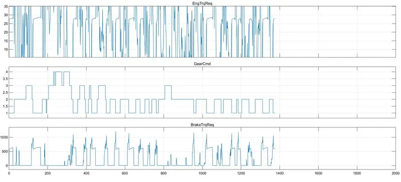
- In this there are three subsystem
- Engine , Transmission,Brake control unit
- Input for engine control unit is Accleration and output is Engine Trq REQ
- Input for brake contro unit is brake and output is Brake Trq Req
ENGINE CONTROL UNIT
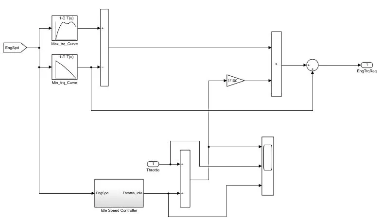
- Input for the Engine Control Unit is EngineSpeed through look up table as maximum torque and speed
- By using second ookup table input as ct torque and mapspeed then it is subtracted and multiplied.
- Output is given as EngTrq req
GRAPH RESULTS
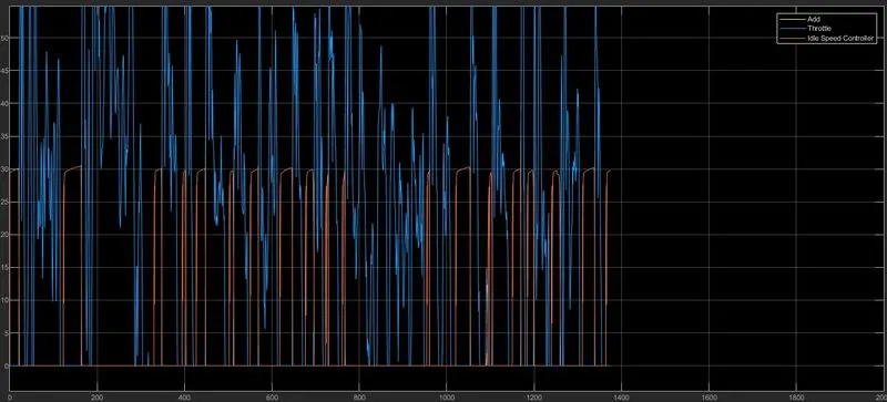
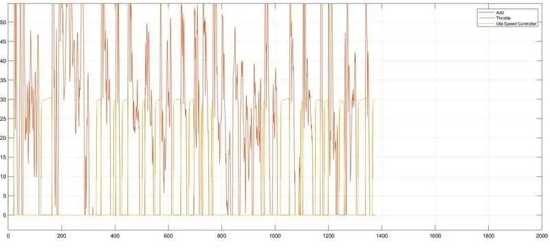
IDLE SPEED CONTROLLER
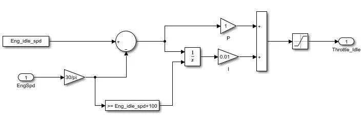
- Input for the idle speed controller is Eng Spd and Engidlespd
- Output is Throttle idle and connected as output scope
TRANSMISSION CONTROL UNIT
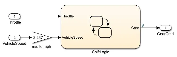
- Input for the Transmission control unit is Throttle and Vehicle Speed
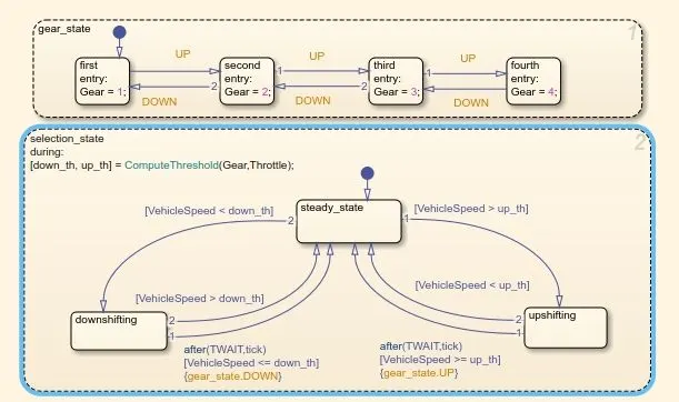
- Steady flow variable state for controlling gears of vehicle with respect to time speed and distance
Shift Logic
BRAKE CONTROL UNIT
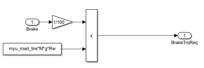
- Calculate brake torque and output is connected through the control signal for powertrain
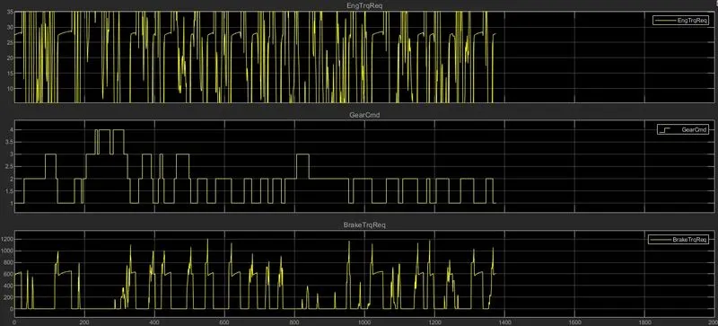
Graph Result
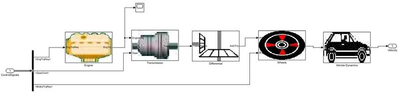
POWERTRAIN
ENGINE
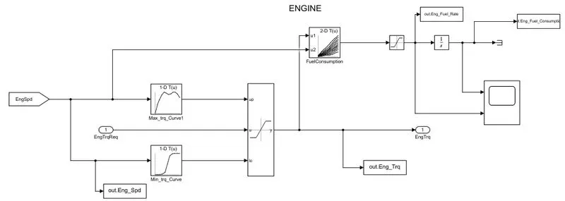
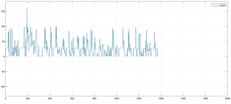
- DiInput is EngTrqReq connected to saturation dynamic block
- Map based model is used for fuel consumption of engine
- Maximum and minimum torque is used from controller and connecte to saturation synamic block
- 2d Look up table is used for fuel consumption ,takes the speed and torque and goes to output as saturatioN
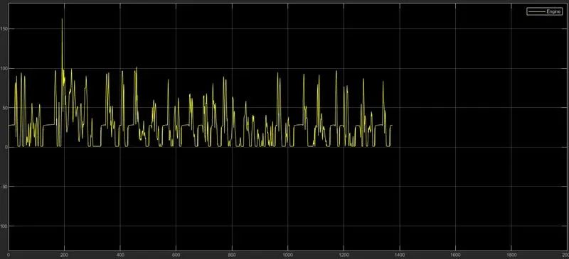
GRAPH RESULT
TRANSMISSION
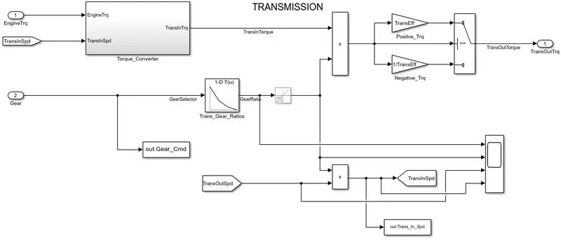
- Input is Engine Torque and Gear from the controller for gear ratio
- Ratio is multiplied input torque , positive and negative torque amd connected to switch as output as tranout trq
- Torque converter is connected engine and transinspd
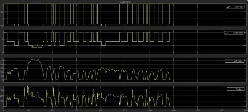
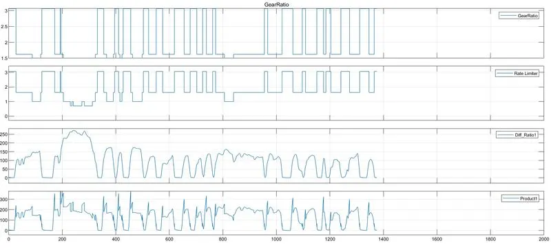
GRAPH RESULTS
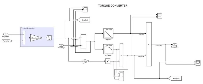
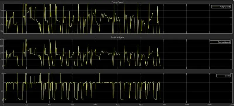
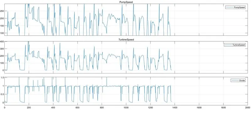
GRAPH RESULT
PUMPSPEED , TURBINE SPEED
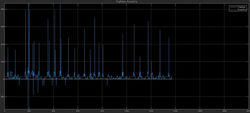
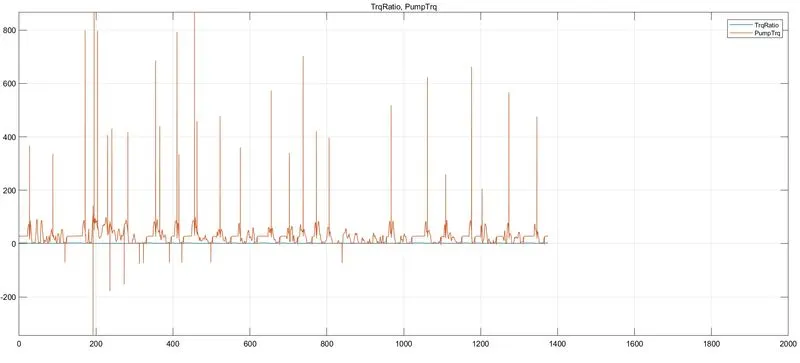
TRQ RATIO, PUMP TRQ
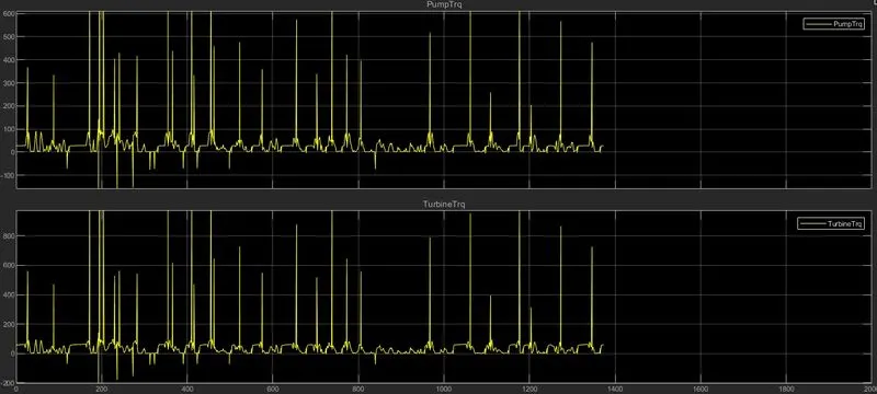
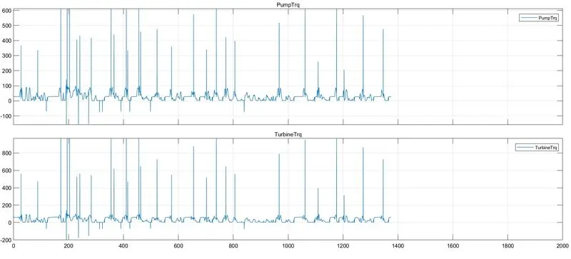
PUMP TRQ , TURBINE TRQ
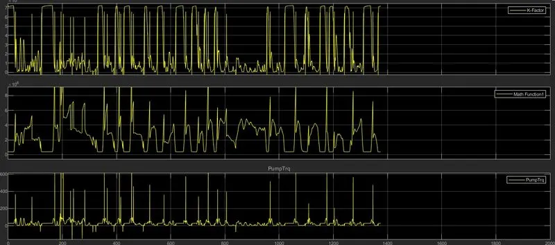
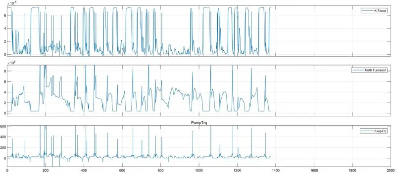
K FACTOR , PUMP TRQ
DIFFERENTIAL
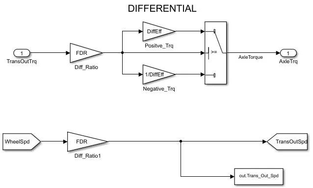
- Input as transmission torque output and connected to Diff ratio for positive and negative torque
- Out put as Axle trq
WHEELS
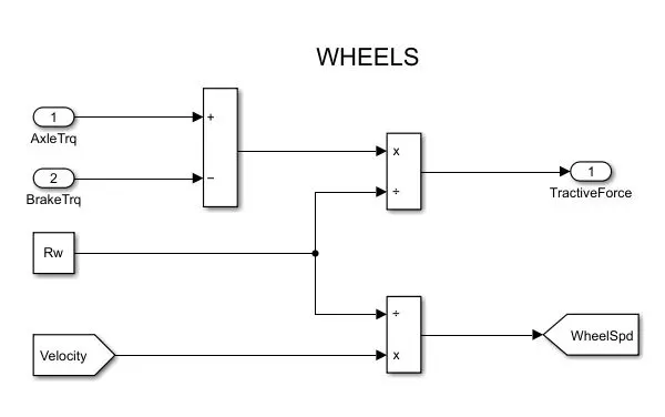
- Input as Axle trq and Brake trq from the controller block
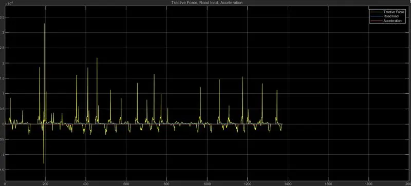
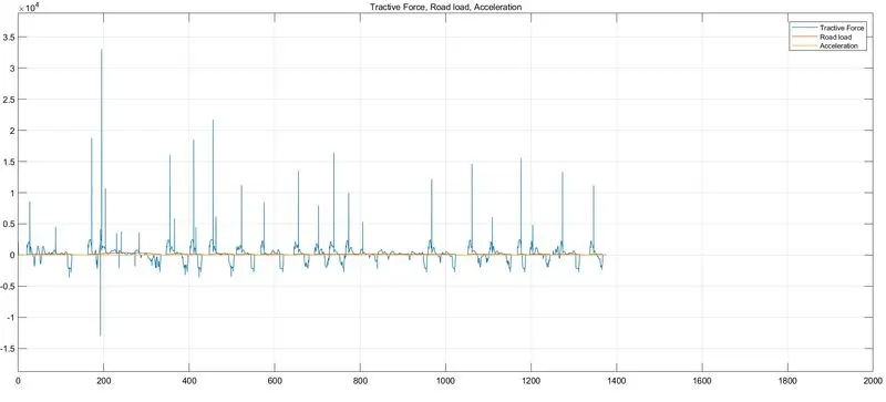
- Subtracted , multiplied rolling radius and velocity and output as Tractive force.
VEHICLE DYNAMICS
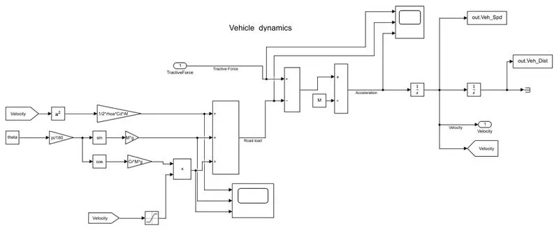

M = Mass kg
A= Frontal area m^2
Cd=Coefficient Drag
Cr= Coefficient of Rolling Resistance
p= Air Density
Vwind=Velocity of wind m/s^2
Vveh= Velocity m/s^2
GRAPH RESULT
CODE
%%%%%%%%%%%%%%%%%%%%%%%%%%%%%%%%%%%%%%%%%%%%%%%%%%%%%%%%%%%%%%%%%%%%%
% Skill-Lync -> Hybrid Drives Development
% Project 1 - Conventional Vehicle Model
% By - VIKAS

% Description:
% The following file is to used with the Initialization file and Simulink
% results for post-processing of the data.
% The file is incomplete, has some examples of how the data is imported
% into a readable format, data analysis and plotting examples.
% Based on the project task, use commands in a similar format as given
% below, to analyse the data and generate required plots.
% You can change variable names if desired

% Post-Processing File
%  File for post-processing the Conventional vehicle simulation model data

% Renaming variables
Time = out.tout;
Acc_Pdl = out.Acc_Pdl;          % Accelerator pedal [%]
Brk_Pdl = out.Brk_Pdl;          % Brake pedal [%]
Gear_Cmd = out.Gear_Cmd;        % Transmission gear
Trans_In_Spd = out.Trans_In_Spd*30/pi;  % Transmission input speed [rpm]
Trans_Out_Spd = out.Trans_Out_Spd*30/pi;% Transmission output speed [rpm]
Eng_Trq = out.Eng_Trq;          % Engine brake torque [Nm]
Eng_Spd = out.Eng_Spd*30/pi;    % Engine speed [rpm]
Eng_Fuel_Consump = out.Eng_Fuel_Consumption;    % Engine fuel consumption [g]
Veh_Dist = out.Veh_Dist/1000;   % Distance traveled by vehicle [km]
Veh_Spd = out.Veh_Spd*18/5;     % Vehicle speed [kmph]
Wheel_Speed = out.wh_speed; % Wheel speed [kmph]
Eng_Fuel_Rate = out.Eng_Fuel_Rate % Engine fuel rate [%]


% Data Analysis
Eng_Pwr = Eng_Spd*pi/30*Eng_Trq/1000;   % Engine brake power [kW]
rho_petrol = 0.7197;                    % Density of petrol [kg/L]
kmpl = Veh_Dist(end)/(Eng_Fuel_Consump(end)/1000/rho_petrol);    % Fuel economy [kmpl]


%TIME VS TRANSMISSION IN OUT SPEED
figure(1)
hold on
grid on
plot(Time, Trans_In_Spd, 'linewidth', 2, 'Color', 'blue');
plot(Time, Trans_Out_Spd, 'linewidth', 2, 'Color', 'green');
ylabel('SPEED [rpm]')
xlabel('TIME [s]')
xlim([0, Time(end)]);
ylim([0, 6000]);
legend('TRANS IN','TRANS OUT');


%  TIME VS ENGINE SPEED TORQUE POWER  FUEL RATE FUEL CONSUMPTION
Eng_spd = Eng_Spd.Data(:,1);              % engine speed
Eng_trq = Eng_Trq.Data(:,1);              % engine torque
Eng_pwr = Eng_Pwr.Data(:,1);              % engine power
Eng_fuel_rate = Eng_Fuel_Rate.Data(:,1);  % engine fuel rate
Eng_fuel_consumption = Eng_Fuel_Consump.Data(:,1); % engine fuel consumption
Veh_dist = Veh_Dist.Data(:,1);            % vehicle distance
Veh_spd = Veh_Spd.Data(:,1);              % vehicle speed


% FUEL ECONOMOY VS FUEL CONSUMPTION
figure(2)
plot(Eng_fuel_consumption,Eng_fuel_rate,'color','G')
xlabel('FUEL CONSUMPTION')
ylabel('FUEL RATE [%]')
title('FUEL ECONOMY Vs FUEL CONSUMPTION')
grid on


% ACCELERATOR , BRAKE PEDAL AND GEAR VS TIME
figure(3)
subplot(2,1,1)
hold on
plot(Time, Acc_Pdl, 'linewidth', 1, 'Color', 'blue');
plot(Time, Brk_Pdl, 'linewidth', 1, 'Color', 'black');
ylabel('Pedal [%]')
xlabel('Time [s]');
xlim([0, Time(end)]);
grid on
legend('ACC','BRAKE');
title('ACCELERATION AND BRAKE PEDAL TIME')
subplot(2,1,2)
plot(Time, Gear_Cmd, 'linewidth', 1, 'Color', 'red');
xlim([0, Time(end)]);
xlabel('TIME [s]');
ylabel('GEAR');
grid on
title('GEAR COMMAND TIME')


% ENGINE SPEED TORQUE POWER FUEL RATE FUEL CONSUMPTION  VS TIME
figure(4)
subplot(2,2,1)
plot(Time,Eng_trq,'linewidth',2,'color','blue')
xlabel('TIME [S]')
ylabel('TORQUE [NM]')
legend('ENGINE TORQUE')
grid on
subplot(2,2,2)
plot(Time,Eng_pwr,'linewidth',2,'color','yellow')
xlabel('TIME [S]')
ylabel('POWER [KW]')
legend('ENGINE POWER')
grid on
subplot(2,2,3)
plot(Time,Eng_fuel_rate,'linewidth',2,'color','green')
xlabel('TIME [S]')
ylabel('FUEL RATE [%]')
legend('ENGINE FUEL RATE')
grid on
subplot(2,2,4)
plot(Time,Eng_fuel_consumption,'linewidth',2,'color','black')
xlabel('TIME [S]')
ylabel('FUEL CONSUMPTION')
legend('ENGINE FUEL CONSUMPTION')
grid on


% ENGINE OPERATING POINTS VS ENGINE FUEL MAP
figure('Name','ENGINE OPERATING POINTS');
hold on
grid on
title('ENGINE OPEARTING POINTS');
p1=plot(Eng_map_spd*30/pi,Eng_max_trq,'linewidth',2,'color','b');
p2=line([Eng_map_spd(end)*30/pi Eng_map_spd(end)*30/pi],[0 Eng_max_trq(end)]);
set(p2,'linewidth',1,'linestyle','--','color','g');
p3=line([Eng_map_spd(1)*30/pi Eng_map_spd(1)*30/pi],[0 Eng_max_trq(1)]);
set(p3,'linewidth',1,'linestyle','--','color','r');
[c,h] = contour(Eng_map_spd'*30/pi,Eng_map_trq,Eng_fuel_map');
clabel(c,h);
xlabel('ENGINE SPEED [rpm]');
ylabel('ENGINE TORQUE [Nm]');
title('ENGINE FUEL CONSUMPTION [G/S]');
legend([p1 p3],{'MAX CURVE','OPERATING POINTS'});
axis([Eng_map_spd(1)*30/pi Eng_map_spd(end)*30/pi 0 Eng_map_trq(end)]);


% GEAR COMMAND VS VEHICLE SPEED
figure(5)
subplot(2,1,1)
plot(Veh_spd, Gear_Cmd, 'linewidth', 1, 'Color', 'yellow');
xlabel('SPEED [RPM]');
ylabel('GEAR');
grid on
title('GEAR VS VEHICLE SPEED')
subplot(2,1,2)
plot(Veh_dist, Gear_Cmd, 'linewidth', 1, 'Color', 'blue');
xlabel('DISTANCE [KMPL]');
ylabel('GEAR');
grid on
title('GEAR VS  DISTANCE')
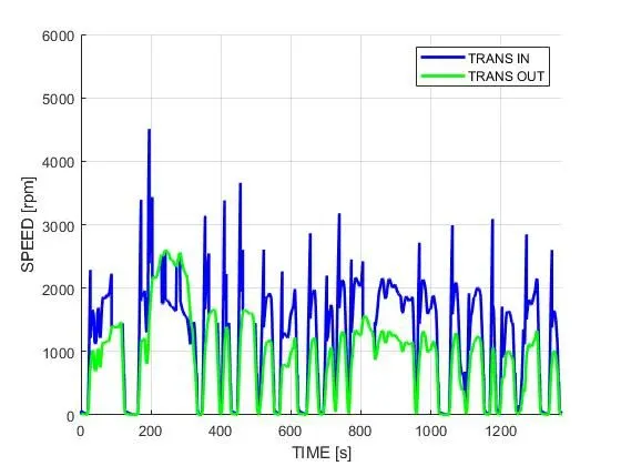
Time vs Transmission INPUT and OUTPUT Speed
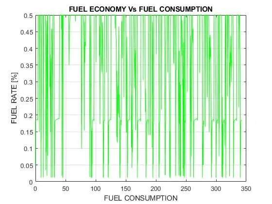
FUEL CONSUMPTION VS FUEL ECONOMY
ACCELERATOR , BRAKE PEDAL VS TIME
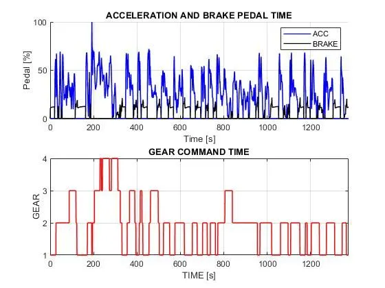
Accleration of vehicle is more compared to brake
ENGINE SPEED TORQUE POWER FUEL RATE FUEL CONSUMPTION VS TIME
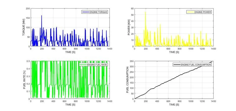
Engine speed torque power fuel rate and fuel consumption is increasing rapidly
ENGINE FUEL CONSUMPTION
GEAR VS VEHICLE SPEED
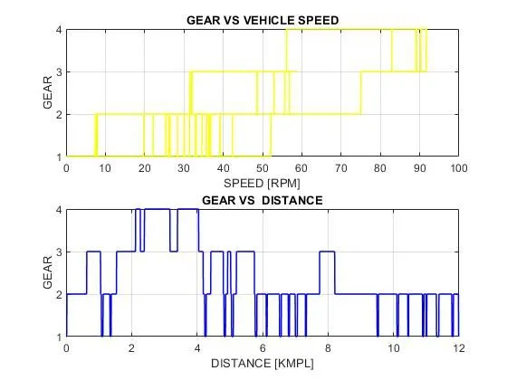
Gear shifting is required as increase vehicle speed
HWFET CYCLE
- Rolling Resistance Aerodynamic drag Power
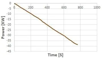
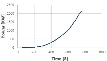
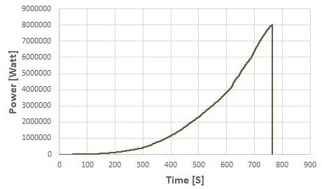
Power increase slowly as increasing aerodynamic drag , Rolling resistance is decreasing
USSD CYCLE
- Rolling Resistance Aerodynamic drag Power
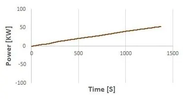
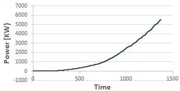
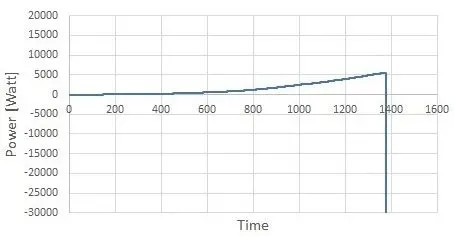
Power is incresed slowly as increasing rolling resistance , aerodynamic drag.