Project 2 - Rankine cycle Simulator

AIM

Writa a code for Rankine cycle using Matlab.

OBJECTIVES

• Calculate the state points for the rankine cycle .
• Plotting the Corresponding T-s and H-s plots for given set of inputs

THEORY

RANKINE CYCLE

The Rankine cycle is an idealized thermodynamic cycle describing the process by which certain heat engines such as steam turbines or reciprocating steam engines allow mechanical work to be extracted from a fluid as it moves between a heat source and heat sink.

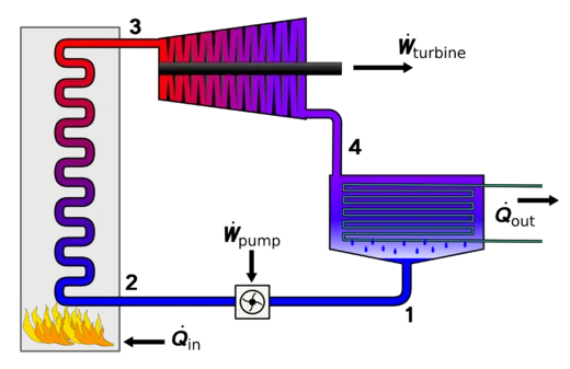
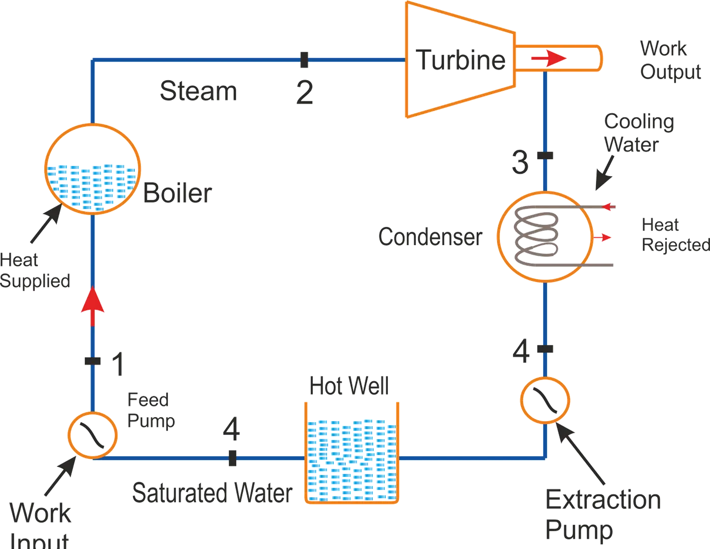
Heat energy is supplied to the system via a boiler where working fluid is converted to a high pressure gaseous state in order to turn a turbine. After passing over the turbine the fluid is allowed to condense back into a liquid state as waste heat energy is rejected before being returned to boiler completing cycle . Friction losses throughout the system are often neglected for the purpose of simplififng calculations as such losses are usually much less significant that thermodynamic losses especially in larger systems.

FOUR PROCESS IN RANKINE CYCLE

PROCESS 1-2

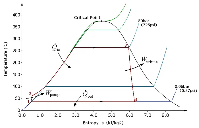
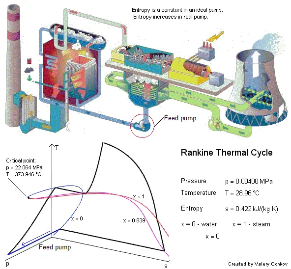
Process 1-2 is Isentropic compression. The working fluid is pumped from low to high pressure . As the fluid is a liquid at this stage the pump require little input energy .

PROCESS 2-3

Process 2-3 is constant pressure heat addition in boiler. The high pressure liquid enters a boiler where it is heated at constant pressure by an external heat source to become a dry saturated vapour. The input energy required can be easily calculated graphically using enthalpy and entropy chart.

PROCESS 3-4

Process 3-4 is isentropic expansion.The dry saturated vapour expands throught a turbine generating power. This decreases the temperature and pressure of the vapour and some condensation may occur. The output in this process can be easily calculated using chart .

PROCESS 4-1

Process 4-1 is a constant pressure heat rejection in condensor. The wet vapour then enters a condensor where it is condensed at a constant pressure to become a saturated liquid .

In an ideal Rankine cycle the pump and turbine would is isentropic the pump and turbine would generate no entropy and hence maximize the network output. Process 1-2 and 3-4 would be represented by vertical lines on T-s diagram and more closely resemble that of the Carnot cycle . The Rankine cycle shows here prevents the state of the working fluid from ending up in the superheated vapour region after the expansion in the turbine which reduces the energy removed by the condensors.

EQUATION

In General the efficiency of a simple rankine cycle can be 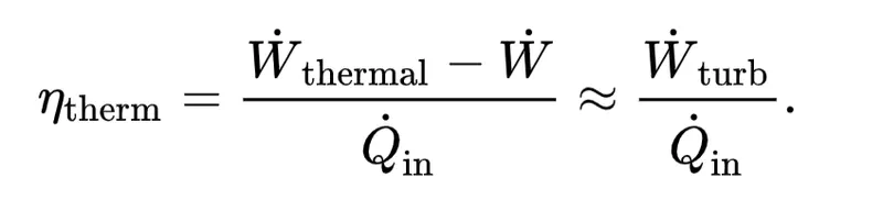Each of the next four equations is derived from the energy and mass balance for a control balance. ntherm defines the thermodynamic efficiency of the cycle as the ratio of net power output to heat input. As the work required by the pump is ofen around 1% of the turbine work output it can be simplifed.

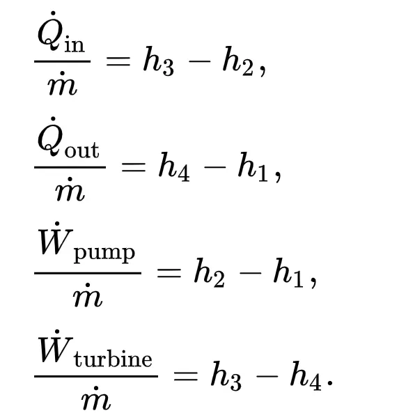
When Dealing with the efficiencies of the turbines and pumps an adjustment to the work terms must be made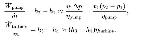

INPUTS

Turbine Inlet temperature = 400° C

Turbine Inlet Pressure = 30 bars

Turbine Outlet Pressure = 0.05 bars = Condenser Inlet Pressure

CODE

% SUBMITTED BY VIKAS
% RANKINE CYCLE SIMULATOR

close all
clear all
clc

% DISPLAY
disp('RANKINE CYCLE SIMULATOR')
disp('1-2 is isentropic expansion in turbine')
disp('2-3 is constant pressure heat rejection in condenser')
disp('3-4 is isentropic compression in pump')
disp('4-1 is constant pressure heat addition in boiler')

% REQUIRED INPUTS
p1=input('enter the pressure at the inlet of turbine (in bar)= ');
t1=input('enter the temp at the inlet of turbine (in degree C)= ');
p2=input('enter the pressure at the inlet of condenser (in bar)= ');


% STEAM CONDITION AT THE INLET TURBINE 
h1=XSteam('h_pt',p1,t1);
s1=XSteam('s_pt',p1,t1);

% STEAM CONDITION AT THE OUTLET TURBINE 
sg2=XSteam('sV_p',p2);
sf2=XSteam('sL_p',p2);
sfg2=sg2-sf2;
x2=(s1-sf2)/sfg2;
s2=sf2+x2*sfg2;
hf2=XSteam('hL_p',p2);
hg2=XSteam('hV_p',p2);
hfg2=hg2-hf2;
h2=hf2+x2*hfg2;
t2=XSteam('Tsat_p',p2);

% WORK DONE BY TURBINE
W_t=h1-h2;

% % STEAM CONDITION AT THE OUTLET CONDESOR 
p3=p2;
t3=XSteam('Tsat_p',p2);
h3=XSteam('hL_p',p2);
s3=XSteam('sL_p',p2);
vf=XSteam('vL_p',p2);
t22=t3;

W_p=vf*(p1-p2)*100;

% STEAM CONDITION AT STATE 4
p4=p1;
h4=W_p+h3;
s4=s3;
t4=XSteam('T_ph',p4,h4);
W_net=W_t-W_p;
Q_s=h1-h4;
Q_r=h2-h3;
efficiency=(W_net/Q_s);

%SPECIFIC STEAM CONDITION
SSC=3600/W_net;
tf_sat=XSteam('Tsat_p',p1);
sf_sat=XSteam('sL_p',p1);
hf_sat=XSteam('hL_p',p1);
sg_sat=XSteam('sV_p',p1);
hg_sat=XSteam('hV_p',p1);


% PLOTTING T-S DIAGRAM
hold on
tsat1=linspace(0,374,1000);
for i=1:length(tsat1)
ss1(i)=XSteam('sL_T',tsat1(i));
end
for j=1:length(tsat1)
ss2(j)=XSteam('sV_T',tsat1(j));
end
plot(ss1,tsat1,'r')
plot(ss2,tsat1,'b')

% SATURATION TEMP AT P1 
temp=XSteam('Tsat_p',p1);
t=linspace(t4,temp,30);
for i=1:length(t)
S(i)=XSteam('s_pt',p1,t(i));
hold on
end
t0=linspace(temp,t1,300);
for i=1:length(t0)
S0(i)=XSteam('s_pt',p1,t0(i));
end
plot([s1 s2],[t1 t2],'y')
text(s1,t1,'1')
text(s2,t2,'2')
plot([s2 s3],[t2 t3],'g','LineWidth',3)
text(s3,t3,'3')
% FOR PUMP WORK
plot([s3 s4],[t3 t4],'b','LineWidth',3)
text(s4,t4,'4')
plot(S,t,'r','LineWidth',3)

% PLOTTING THE PHASE CHANGE REGION 
plot([sf_sat sg_sat],[tf_sat tf_sat],'g','LineWidth',3)
plot(S0,t0,'y','LineWidth',3)
legend('SATURATION CURVE L','SATURATION CURVE  V','TURBINE','CONDESOR','PUMP','BOILER',)
title('T-S DIAGRAM')
xlabel('ENTROPY')
ylabel('TEMPERATURE')

% PLOTTING H-S DIAGRAM
figure(2)
hold on
tsat1=linspace(0,374,1000);
for i=1:length(tsat1)
hh1(i)=XSteam('hL_T',tsat1(i));
end
for j=1:length(tsat1)
hh2(j)=XSteam('hV_T',tsat1(j));
end
plot(ss1,hh1,'r')
plot(ss2,hh2,'b')

% PLOTTING TURBINE
plot([s1 s2],[h1 h2],'k','LineWidth',3)
text(s1,h1,'1')

% PLOTTING CONDESOR
plot([s2 s3],[h2 h3],'y','LineWidth',3)
text(s2,h2,'2')

% PLOTTING PUMP 
plot([s3 s4],[h3 h4],'m','LineWidth',3)
text(s3,h3,'3')
s=linspace(s3,s1,1000);
for i=1:length(s)
h(i)=XSteam('h_ps',p1,s(i));
end

% PLOTTING BIOLER
% plot([s4 s1],[h4 h1],'y')
plot(s,h,'r')
legend('SATURATION CURVE L','SATURATION CURVE  V','TURBINE','CONDESOR','PUMP','BOILER','Location','southwest')
title('H-S DIAGRAM')
xlabel('ENTROPY')
ylabel('ENTHALPY')

% OUTPUTS
% STATE 1
fprintf('At State Point 1:\r\n')
fprintf('P1 is : %f Bar\r\n',p1)
fprintf('T1 is : %f Deg Celcius\r\n',t1)
fprintf('H1 is : %f KJ/Kg\r\n',h1)
fprintf('S1 is : %f KJ/KgK\r\n',s1)

% STATE 2
fprintf('At State Point 2:\r\n')
fprintf('P2 is : %f Bar\r\n',p2)
fprintf('T2 is : %f Deg Celcius\r\n',t2)
fprintf('H2 is : %f KJ/Kg\r\n',h2)
fprintf('S2 is : %f KJ/KgK\r\n',s2)
fprintf('X is : %f \r\n',x2)

% STATE 3
fprintf('At State Point 3:\r\n')
fprintf('P3 is : %f Bar\r\n',p3)
fprintf('T3 is : %f Deg Celcius\r\n',t3)
fprintf('H3 is : %f KJ/Kg\r\n',h3)
fprintf('S3 is : %f KJ/KgK\r\n',s3)

% STATE 4
fprintf('At State Point 4:\r\n')
fprintf('P4 is : %f Bar\r\n',p4)
fprintf('T4 is : %f Deg Celcius\r\n',t4)
fprintf('H4 is : %f KJ/Kg\r\n',h4)
fprintf('S4 is : %f KJ/KgK\r\n',s4)

% CALCULATIONS
fprintf('Work Done By Turbine : %f kJ/kg\r\n',W_t)
fprintf('Work Done By Pump : %f kJ/kg\r\n',W_p)
fprintf('Heat Added in The Boiler: %f KJ/kg\r\n',Q_s)
fprintf('Heat Rejected in The Condenser: %f KJ/kg\r\n',Q_r)
fprintf('Thermal Efficiency is : %f %%\r\n',efficiency*100)
fprintf('Specific Steam Consumption : %f KJ/kWh\r\n',SSC)

• Xstream data is used to extract steam and water properties of enthalpy , entropy at specific pressure and temperature for sat liquid sat vapour conditions
• The program requires the input of pressure in bar at state 1 (turbine inlet) Temperature at same point (deg celcius ) and temp at condensor inlet point 2
• With the help of these inlets rom Xstream data the program calculates all the state points of the rankine cycle.
• As we extract data we use thermodynamic relation to further find state points and extract thier data from Xstream
• sf and sg , hf , hg where f and g stands for saturated liquid and saturated vapour respectively
• Efficiency and Specific steam consumption of the rankine is calculated
• Saturation curve is plotted in for saturated liquid and saturated gas
• Plot t vs s and h vs s is created froma all points obtained from the program
• The plot changes as the user input changes to above mentioned inputs
• Results are displayed in command window

RESULTS AND OUTPUT

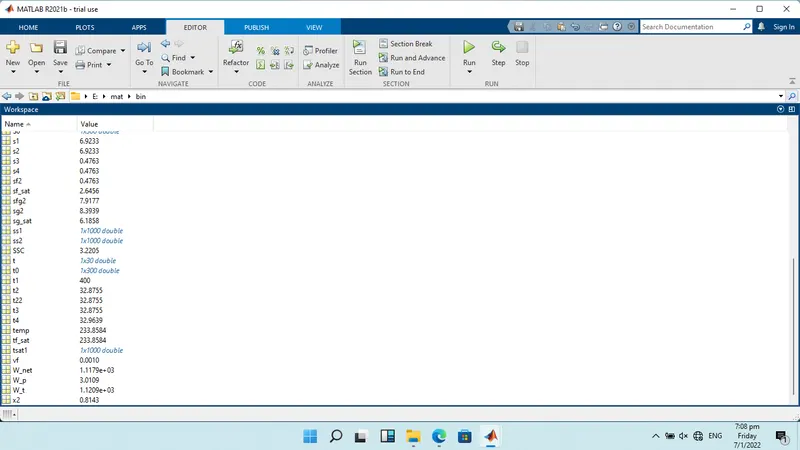
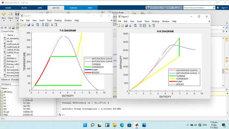
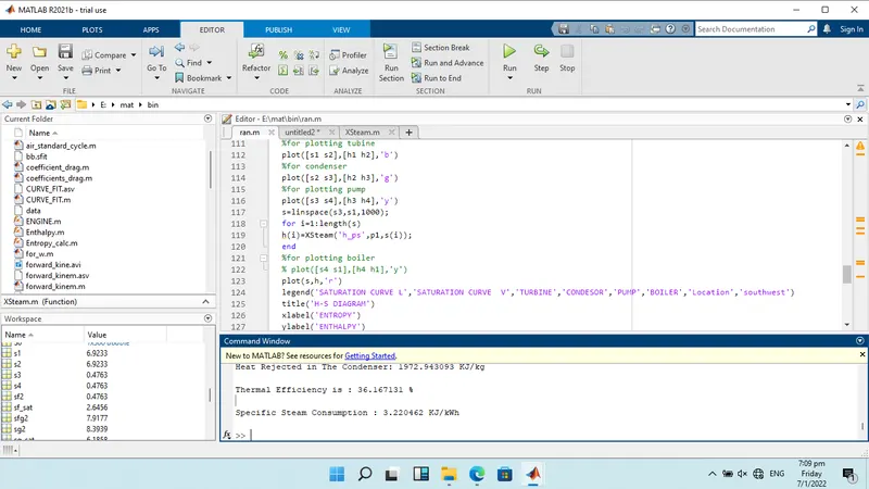
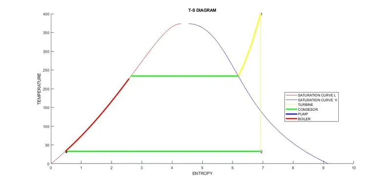
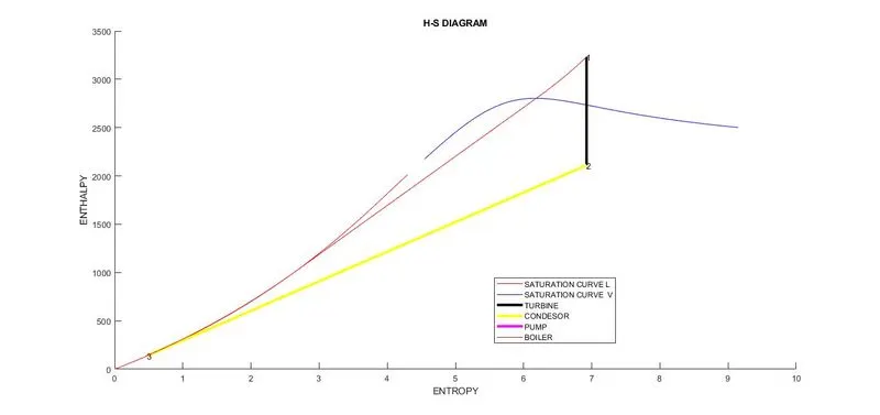
OUTPUT

RANKINE CYCLE SIMULATOR
1-2 is isentropic expansion in turbine
2-3 is constant pressure heat rejection in condenser
3-4 is isentropic compression in pump
4-1 is constant pressure heat addition in boiler
enter the pressure at the inlet of turbine (in bar)= 30
enter the temp at the inlet of turbine (in degree C)= 400
enter the pressure at the inlet of condenser (in bar)= 0.05
At State Point 1:

P1 is : 30.000000 Bar

T1 is : 400.000000 Deg Celcius

H1 is : 3231.571027 KJ/Kg

S1 is : 6.923259 KJ/KgK

At State Point 2:

P2 is : 0.050000 Bar

T2 is : 32.875490 Deg Celcius

H2 is : 2110.708212 KJ/Kg

S2 is : 6.923259 KJ/KgK

X is : 0.814256 

At State Point 3:

P3 is : 0.050000 Bar

T3 is : 32.875490 Deg Celcius

H3 is : 137.765119 KJ/Kg

S3 is : 0.476254 KJ/KgK

At State Point 4:

P4 is : 30.000000 Bar

T4 is : 32.963884 Deg Celcius

H4 is : 140.776056 KJ/Kg

S4 is : 0.476254 KJ/KgK

Work Done By Turbine : 1120.862815 kJ/kg

Work Done By Pump : 3.010937 kJ/kg

Heat Added in The Boiler: 3090.794971 KJ/kg

Heat Rejected in The Condenser: 1972.943093 KJ/kg

Thermal Efficiency is : 36.167131 %

Specific Steam Consumption : 3.220462 KJ/kWh

>> 

ERROR

CONCLUSION

The rankine cycle is closed by a condensor using cooling water that convert saturated vapor at low pressure from the turbine generator into condensate which is pumped back to the heat exchanger to restart cycle.