Week 3 - Solving second order ODEs
AIM
To solve second order differential equation (ODE) using Matlab.
OBJECTIVES
- To solve the second order ODE with graph of Velocity v/s Displacement.
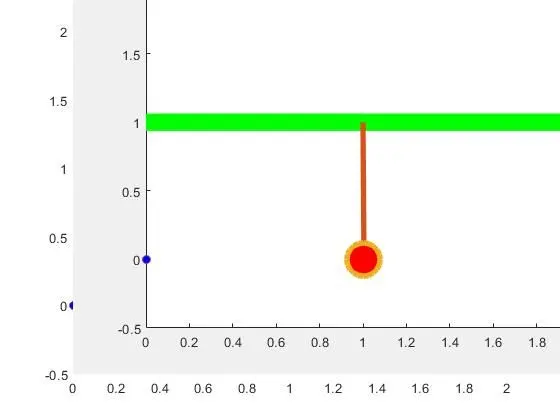
- To create the animation of the simple pendulum.
THEORY
Ordrinary Differential Equation An ordinary differential euation(ODE) is the differential equation containing one or more functions of one independent variables and derivates of those functions. The term ordinary is used in constrast with the term partial difference which may be respect to more than one independent variable.
SIMPLE PENDULUM
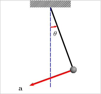
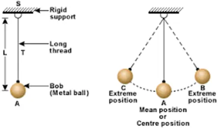
The Simple Pendulum is an idealized mathematical model of a pendulum. Thus a weight for bob on the massless cord suspended from apivot without friction. When given an intial push it will swing back and forth at a constract amplitude . Real pendulum are subject to friction air during the swing decreases.
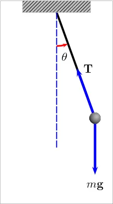
Govering Equation
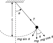
Theta is the angle made by the movable link with vertical axis.
L is the length of the movable rod
m is the mass of the bob
b is the damping coefficient of the system.
1.  second order ODE -------------(1)
To solve this ODE we need to reduce the order of equation into lower order.
theta=theta1 so that implies
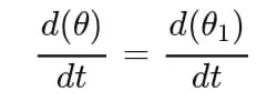 = theta2---------------(2)
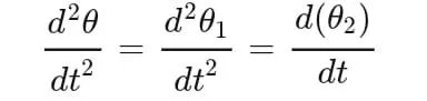 ---------------(3)
Putting the value of (2) and (3) in (1) we get
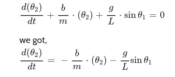
INPUTS
Simulate the motion between 0-20 sec
t=0
L=1m
M=1kg
b=0.05
g=9.81m/s2
Angular velocity= 3 rad/sec
PROGRAM
function [dtheta_dt]=ode_func(t,theta,b,g,l,m)


theta1=theta(1);
theta2=theta(2);
dtheta1_dt=theta2;
dtheta2_dt=-(b/m)*theta2-(g/l)*sin(theta1);

dtheta_dt=[dtheta1_dt;dtheta2_dt]

end
MAIN PROGRAM
% SUBMITTED BY VIKAS
% MOTION OF PENDULUM

clear all
close all
clc

% INPUT VARIABLES FOR SECOND ORDER ODE OF A SIMPLE PENDULUM

b=0.05;
g=9.81;
l=1;
m=1;

theta_0=[0;3]
omega_0=3

t_span=linspace(0,20,500);

% ODE 45 FUNCTION SOLVE SECOND ORDER ODE
[t,results]=ode45(@(t,theta)ode_func(t,theta,b,g,l,m),t_span,theta_0);


% PLOTTING OF ANGULAR VELOCITY AND DISPLACEMENT
figure(1)
hold on
plot(t,results(:,1))
plot(t,results(:,2))
grid on
xlabel('TIME IN SECONDS')
ylabel('ANGULAR VELOCITY(RAD/S)/DISPLACEMENT(RAD)')
legend('Displacement','Angular velocity')
title('MOTION OF PENDULUM')


angle=results(:,1);

% COUNT COMMAND FOR ITERATIONS
ct=1;

for i=1:length(angle);

    % FIXED COORDINATES OF ONE END OF SIMPLE PENDULUM
    x0=0
    y0=0

    % MOVING COORDINATES OF THE BOB
    x1=1-l*sin(angle(i));
    y1=1-l*cos(angle(i));

    % PLOTTING BOB MOTION
    figure(2)
    plot([0 2],[1 1],'LineWidth',13,'color','g')
    hold on
    plot([1 x1],[1 y1],[x1 x1],[y1 y1],'o','markersize',25,'MarkerFaceColor','r','LineWidth',4)
    plot(x0, y0,'-o','markerfacecolor','b')
    axis([0 2 -0.5 2])
    M(ct)=getframe(gcf);
    ct=ct+1;
    hold off
end

% TO CREATE A ANIMATION OF THE SIMPLE PENDULUM
movie(M)
videofile=VideoWriter('SIMPLE_PENDULUM.avi','Uncompressed AVI');
open(videofile)
writeVideo(videofile,M)
close(videofile)
RESULTS
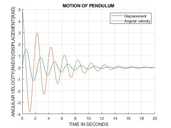
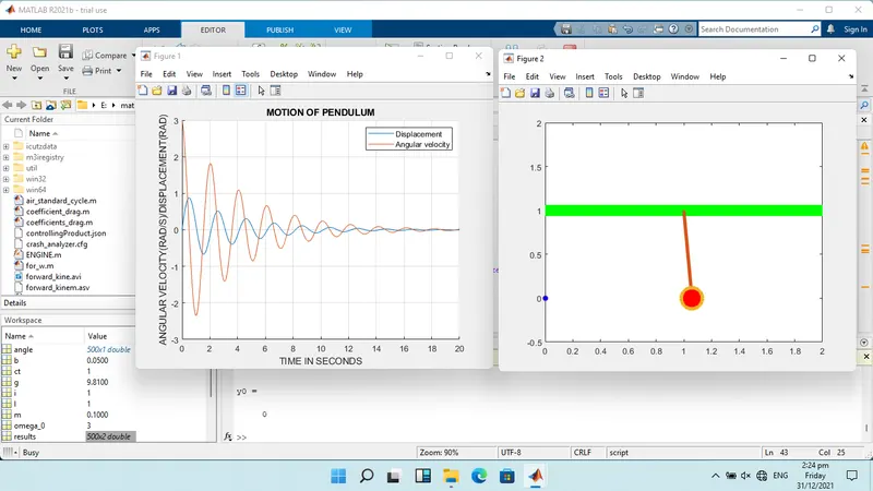
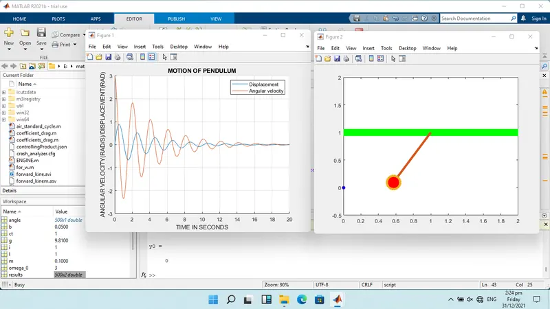
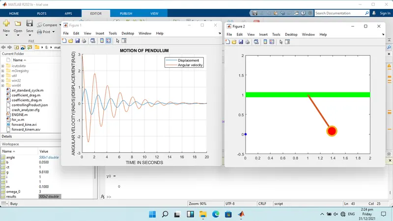
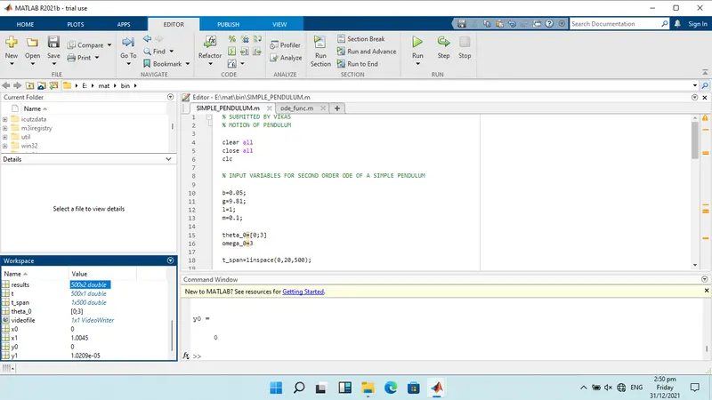
Graph for velocity vs time which shows displacement and angular velocity.
SIMULATION
Errors

Conclusion
- The graph of displacement and angular velocity is plotted in velocity vs time.
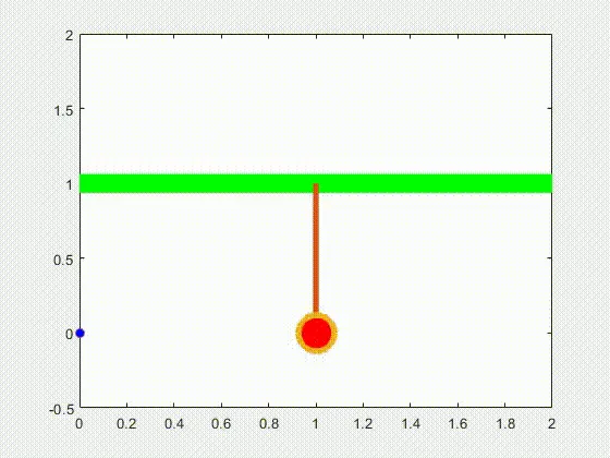
- Animation of simple pendulum.
Link
https://drive.google.com/file/d/1ocG8l3-cPd3YfxMWDVg77_N5Hw7XxUUT/view?usp=sharing