Week 4.1 - Genetic Algorithm

AIM

To optimize the stalagmite function and find the global minimum of function.

OBJECTIVES

Explaining the concept of genetic algorithim and also ga synatx.

THEORY

OPTIMIZATION

Optimization is the process of making something better . In any process we have st of inputs a set of outputs as

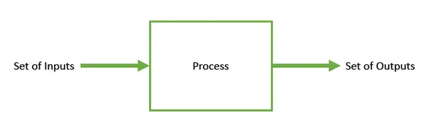
Optimization refers to finding the values of inputs in such a way that we get the best output values.The definition of best varies rom problem to problrm but in mathemaical terms it refers to maximizing or minimizing one or more objective functions by varying the input parameters.

GENETIC ALGORITHIM

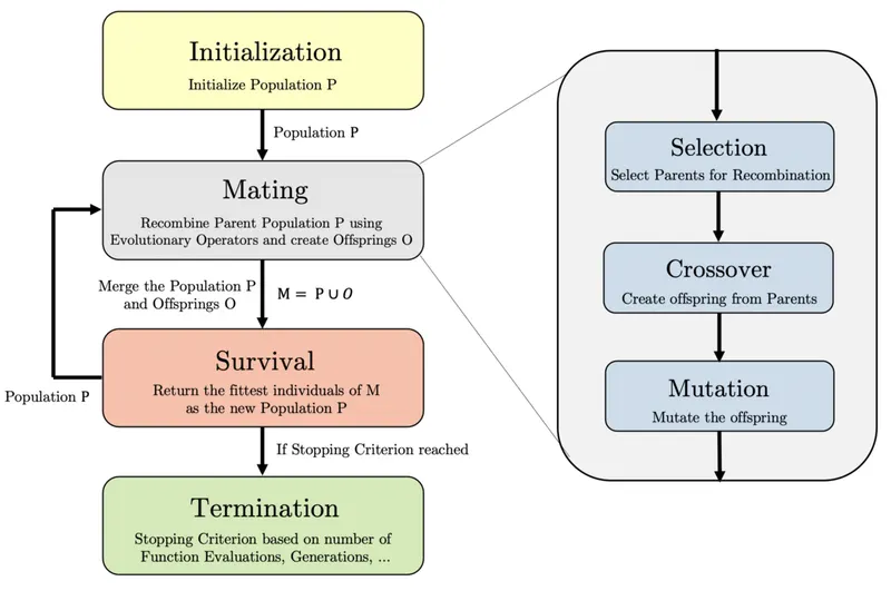
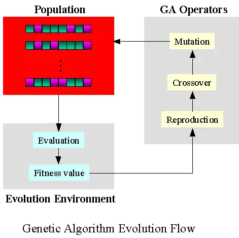
Genetic algorithim is a search heurstic that is inspired by Charles Darwin thoery of natural evolution. This Alogrithim reflects the process of natural selection where fittest individuals are selected for reproduction to generate offsprings for next generation.

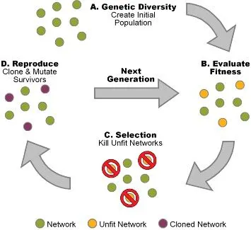
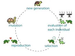
PROCESS OF NATURAL SELECTION

• This process starts with selection of fittest individual form a given set of population.
• They produce offsprings which inherit the characterstics of the parent and will be added to next generation.
• If the parents are fit enough thier offsprings will be better thier parents and will have better chance of surviving.
• This process keeps on iterating and the end a generation of fittest individuals will be obtained.
• This Whole notion can be helpful in search problems.
• We select a set of solutions to a problem and sort out a set of best ones out of them . This will eventually narrow down to one best solution that gives optimum result for given problem.

FIVE PHASES IN GENETIC ALGORITHM

1. Intial Population

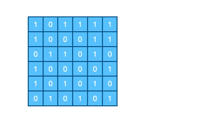
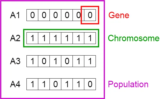
The problem intiates with a set of individuals whic is called population. Each individual is a solution to the problem we want to solve . Each individual is characterized by a set of parameters called genes.

Genes are joined into a string which yields us chromosome which is nothing but a solution.

2. Fitness function

The fitness fnction determines how fit an individual and gives a fitness score to each individual. The probablity that an individual will be selected for reproduction is based on this score.

3. Selection phase

The main objective of this phase is to select the fittest individual and let them pass thier gene onto the next generation.

4. Cross over

For each pair of parents to be mated crossover points is chosen at random from within the genes .

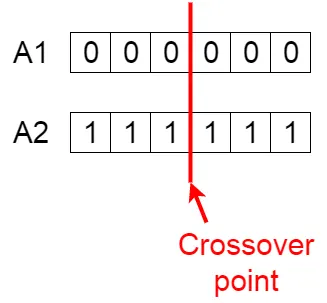
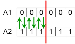
Off springs are created by exchanging genes of parents among themselves until the crossover point is reached.

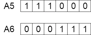
The New offspring is then added to the population.

5. Mutation

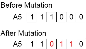
In certain newoffsprings formed some of thier genes can be subjected to the mutation with the low random probablity.This Implies that some of the bits in the bitstring can be flipped.

STRUCTURE

ADVANATGES OF GA

• Does not require any deriavative information
• Is faster and more efficient as compared to the tradional way methods.
• Has very good parallel capabalities.
• Optimize both continues and discrete function and also multi-objective problems.
• Provide a list of good solutions not just a single solution .
• Always get an answer to the problem which gets better over the time.
• Useful when the search space is very large and there are large number of parameters involved.

LIMITATION OF GA

• GA are not suited for all problems especially problems which are simple and for which derivative information is available.
• Fitness value is calculated repeatedly which might be computationally expensive for some problems.
• Being stochastic there are no guarentees on the optimality or the quality of the solution.
• If not implemented properly the GA may not converge to the optimal solution.

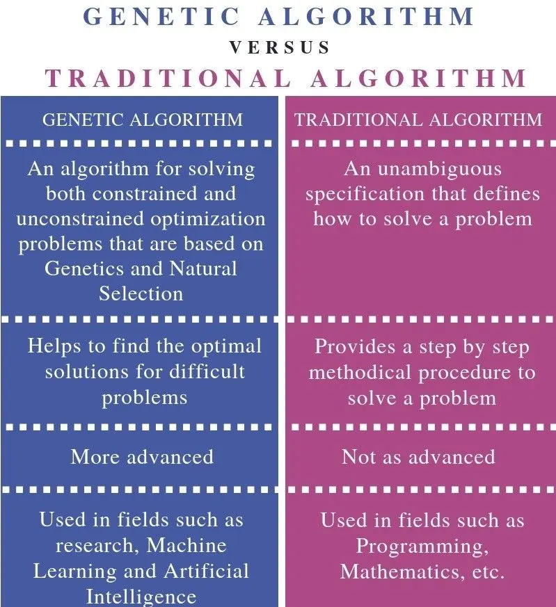
DIFFERENCE

PSEUDOCODE

START
Generate the initial population
Compute fitness
REPEAT
    Selection
    Crossover
    Mutation
    Compute fitness
UNTIL population has converged
STOP

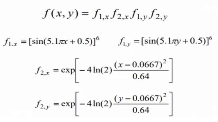
FITNESS FUNCTION

The format for writing genetic algorithim in MATLAB

x = ga(fun,nvars,A,b,Aeq,beq,lb,ub,nonlcon,options)

1. x is the local minima point.

2. fun is the function to be called ( its the stalagmite function)

3. nvars indicate dno variables used.

4. A and b are used to indicate any kind inequalties that exist in function.

5. Aeq and Beq also denotes the inequalities.

6. lb-Lower bound.

7. ub- Upper bound.

8. nonclon gives a two vector representing inequalities and equalities.

9. options is used to perform additional operations like increasing population size . This is done with the help of optimoptions.

STALAGMITE FUNCTION

function [F] = stalagmite(input_vector)
 x = input_vector(1);
 y = input_vector(2);
 f1=(sin(5.1*pi*x + 0.5)).^6;
 f2=(sin(5.1*pi*y + 0.5)).^6;
 f3= exp((-4*log(2)*(x-0.0667).^2)/(0.64));
 f4= exp((-4*log(2)*(y-0.0667).^2)/(0.64));
 F = -f1*f2*f3*f4;
end

While using the function at the end as we are using the -ve sign so that the plot will be reversed as we have to find the maxima of the given function using GA.

MAIN FUNCTION

% SUBMITTED BY VIKAS
% GENETIC ALGORITHIM
clear all 
close all
clc 

x = linspace(0,0.6,150);
y = linspace(0,0.6,150);
iterations = 50;
% CREATING 2D MESH
[xx, yy] =meshgrid(x,y);


% EVALUATING STALAGMITE FUNCTION
for i=1:length(xx)
 for j = 1:length(yy)
 input_vector(1) = xx(i,j);
 input_vector(2) = yy(i,j);
 f(i,j) = stalagmite(input_vector);
 end
end


% UNBOUNDED STATICAL BEHAVIOUR
tic 
for i=1:iterations
[inputs , f_opt(i)] = ga(@stalagmite,2);
x_opt(i) = inputs(1);
y_opt(i) = inputs(2);
end
iteration_1_time = toc
% PLOTTING
figure (1)
subplot(2,1,1)
hold on
surfc(xx,yy,f)
shading interp
plot3(x_opt,y_opt,f_opt,'marker','o','markersize',5,'markerfacecolor','b')
xlabel('X VALUE')
ylabel('Y VALUE')
zlabel('FUNCTION VALUE ')
title('UNBOUNDED STATICAL BEHAVIOUR')
subplot(2,1,2)
plot(f_opt)
xlabel('ITERATIONS')
ylabel('FUNCTION MAXIMUM')



% STATISTICAL BEHAVIOUR WITH UPPER AND LOWER LIMIT
tic
for i=1:iterations
[inputs , f_opt(i)] = ga(@stalagmite,2,[],[],[],[],[0;0],[1;1]);
x_opt(i) = inputs(1);
y_opt(i) = inputs(2);
end
iteration_2_time = toc
%plotting
figure (2)
subplot(2,1,1)
hold on
surfc(xx,yy,f)
shading interp
plot3(x_opt,y_opt,f_opt,'marker','o','markersize',5,'markerfacecolor','b')
title('BOUNDED STATICAL BEHAVIOUR')
xlabel('X VALUE')
ylabel('Y VALUE')
zlabel('FUNCTION VALUE ')
subplot(2,1,2)
plot(f_opt)
xlabel('ITERATIONS')
ylabel('FUNCTION MAXIMUM')




% INCREASING GA POPULATION SIZE  
options = optimoptions('ga');
options = optimoptions(options,'populationsize',200)
tic
for i=1:iterations
[inputs , f_optimum(i)] = ga(@stalagmite,2,[],[],[],[],[0;0],[1;1],[],[],options);
x_optimum(i) = inputs(1);
y_optimum(i) = inputs(2);
end
iteration_3_time = toc

% PLOTTING
figure (3)
subplot(2,1,1)
hold on
surfc(xx,yy,f)
shading interp
plot3(x_optimum,y_optimum,f_optimum,'marker','o','markersize',5,'markerfacecolor','b')
title('BOUNDED STASTICAL BEHAVIOUR WITH INCREASED POPULATION SIZE ')
xlabel('X VALUE')
ylabel('Y VALUE')
zlabel('FUNCTION VALUE ')
subplot(2,1,2)
plot(f_optimum)
xlabel('ITERATIONS')
ylabel('FUNCTION MAXIMUM')

MAIN FUNCTION

• Firstly creating the mesh from the two vectors which will be acting as search space to find the maxima of the function.
• Creating the mesh of these two vectors using the mesh command and defining the no of iterations as num_cases to iterate the values of the optimum values of the function.
• Now calculating the values of the fitness function at each point of mesh grid is formed.
• Now creating its surface through surfc command which will also provide contour of the generated surface.
• While using surfc applying the -ve sign to the function will be generated the surfaced upside down which will be quite control to get the maxima of the function as will provide positive value for the ,maximum using the -ve sign.

1st iteration

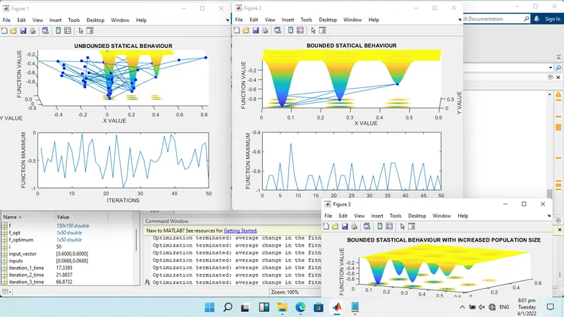
In the first iteration the behaviour of the algorithim is studied by not defining the limits. The GA does not run within a particular search space since we have not defined bounds.

2nd iteration

Here the lower and upper bounds are defined so as to know the boundaries within which the global maxiam lies.In other words we are defining space within which the global maxima is to be found.

3rd iteration

In this iteration the population size is increased so as to converge the global minima.

RESULTS AND CONCLUSION

1ST ITERATION

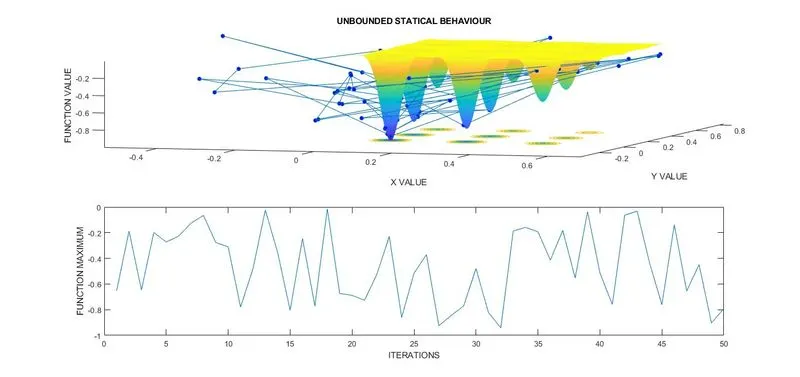
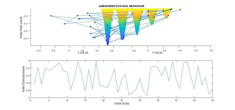
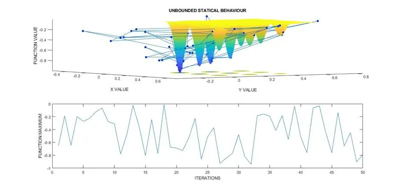
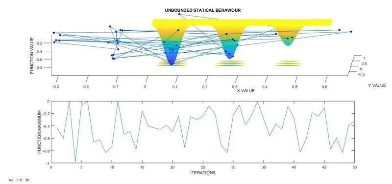
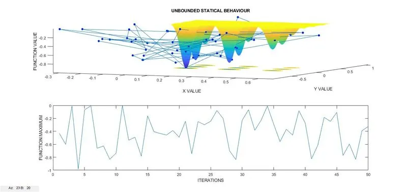
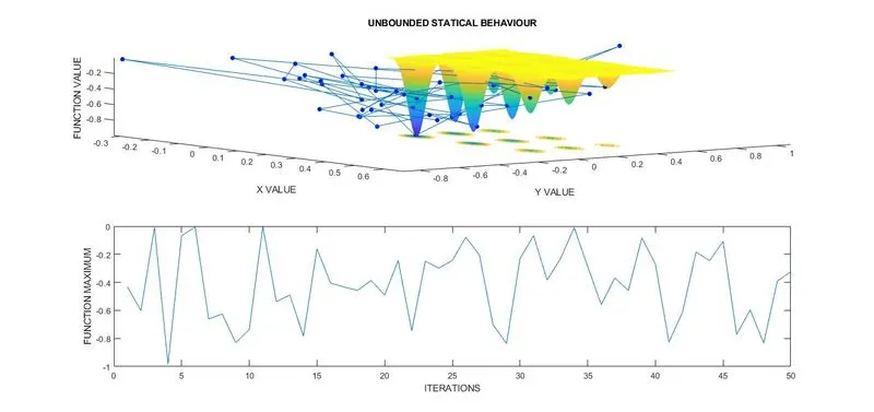
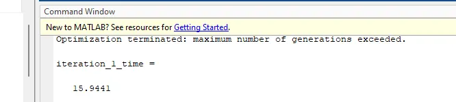
It can be seen that since the inputs are unbound GA algorithim has mapped local maxima points outside our stalagmite function.

2nd ITERATION

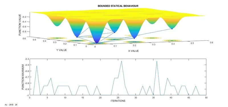
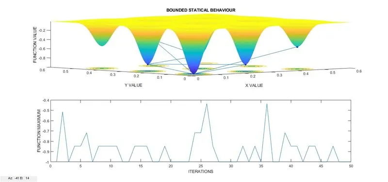
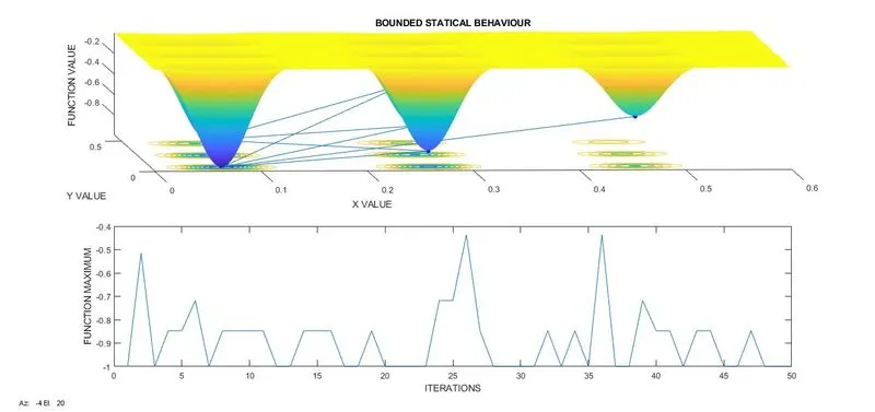
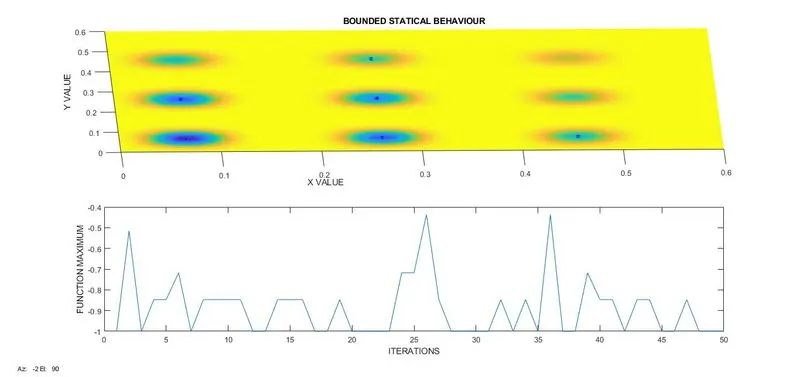
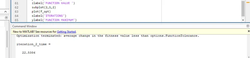
Graph is more clear optimised compared to 1st iteration since here the bounds were defined and we could get only the values within our range . We now more clear on the range within which our maxima lies.

3rd ITERATION

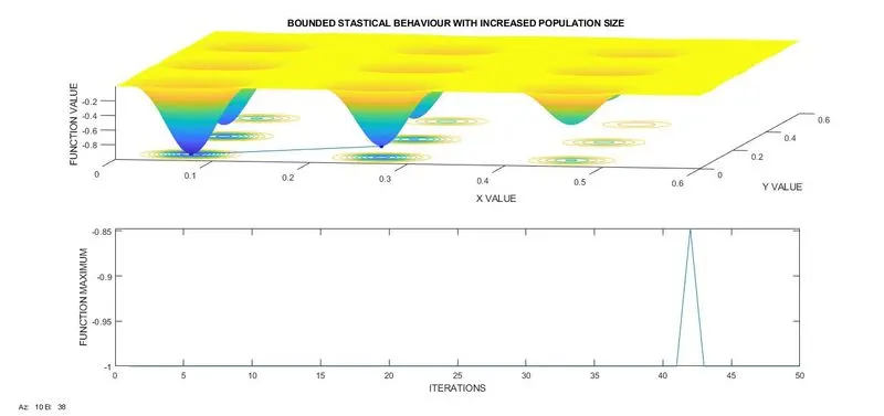
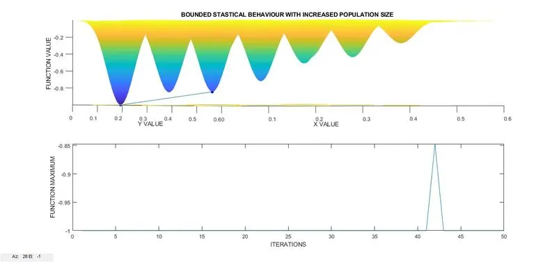
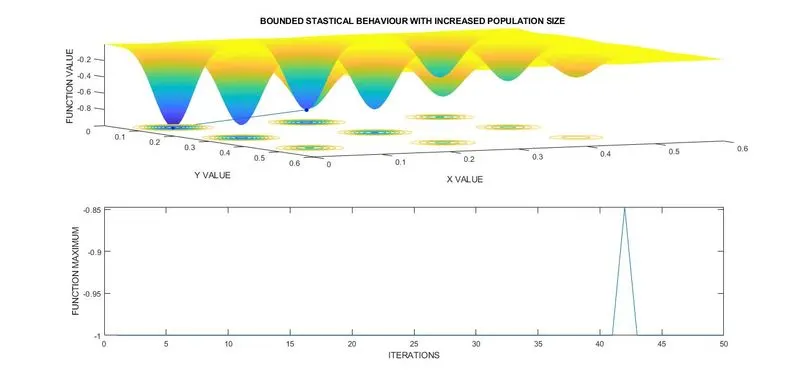
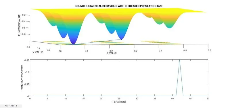
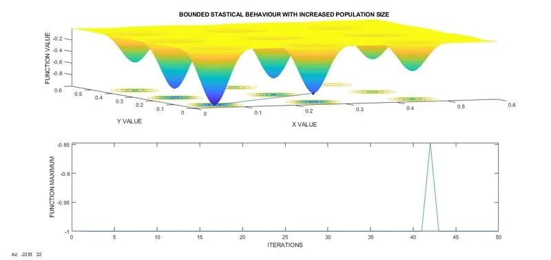
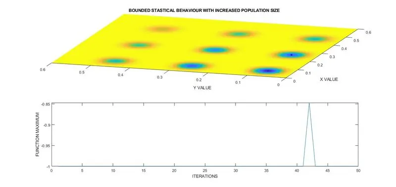
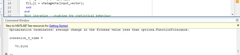
We are getting the optimise dvalue of a global maxima with the accurate range since the incresed number of iterations and population size. Since the number of iterations and population size is incresed the study size is high compared to previous two iterations.

Thus it can be concluded that GA gives more accurate results in case of bounded inputs and by increasing number of iterations and population size.

REFERENCES

1. https://towardsdatascience.com/introduction-to-genetic-algorithms-including-example-code-e396e98d8bf3

2. https://in.mathworks.com/discovery/genetic-algorithm.html