Project 1
Table of contents
- Objective of study
- Problem statement
- Theoretical study
3.1 Types of propulsion Models
3.2 Conventional or IC Engines
3.3 Forward Based Conventional Vehicle Model
- Formulae used for computation and modelling
- Project Overview
5.1 Matlab prerequisites for modelling
5.2 Matlab pre-processing code
5.3 Simulink Model and its subsystems
5.3.1 Driver Subsystem
5.3.2 Controller Unit
5.3.3 Engine
5.3.4 Transmission
5.3.5 Differential
5.3.6 Wheels
5.3.7 Vehicle Dynamics
5.4 Post processing Matlab code
- Results
- Conclusion
- References
01.Objective:
Model a forward energy based fuel consumption model of a conventional vehicle using matlab and Simulink. Based on the model we will study
- Fuel consumption map of HWFET and UDDS cycles.
- Analyse and understand engine operating points in terms of engine speed, torque, transmission speeds pedal positions, gears distance travelled.
- Load results into Matlab.
- Plot time trace for engine, transmission input, transmission output and wheel speed.
- Plot engine torque, engine power, rate of fuel consumption and total fuel consumption.
- Plot accelerator and brake pedal, gear command vehicle desired and actual speed total distance.
02.Problem Statement:
We have a typical midsize car with a 1.9L engine and a 4 speed automatic transmission is considered. Data is taken from ADVISOR data base developed by NREL, USA. Transmission shift map and controller is taken from Matlab/Simulink example database.
The model is loaded with data for different drive cycles like UDDS, HWFET, FTP, NEDC,US06 and WLTP and it has a capability simulate all these drive cycles.
The Simulink model has a driver block, controller unit and a power train. The subsystem are created within the block as per requirement and we will be discussing each one in details in coming pages. We have a following task to be done before executing the code and model to obtain the results
- We have an incomplete Simulink model of forward energy based fuel consumption conventional vehicle model where engine block and vehicle blocks needs to be modelled.
- Provided input data in the form of matlab code which can be run and data can be stored in workspace.
- After completing the model the results needs to be sent to workspace using to workspace command and stored.
- The obtained results to be used to plot the results and analyse them.
- We need to find the fuel efficiency of the vehicle for HWFET and UDDS drive cycles.
03.Theoretical study:
3.1 Types of Propulsion Models
Based on energy source used we can classify the vehicle models as below,
Conventional vehicles use an internal combustion engine fuelled by gasoline or diesel to power the wheels. Electricity is used for some accessories, but is not used to move the vehicle.
Vehicles can be powered in several different ways, from gasoline to electric batteries and a spectrum of choices in between.
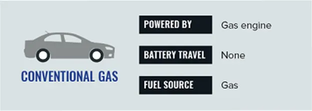
Fig 01. Conventional Vehicle
Conventional hybrids, also referred to as hybrid electric vehicles (HEVs), supplement the internal combustion engine with electrical power produced by an on-board electric motor. The electrical system acts as a generator when a driver applies the brakes, converting kinetic energy into electrical energy that is stored in a small battery pack. The primary fuel is gasoline or diesel.
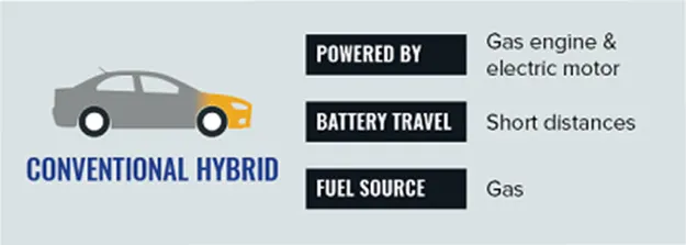
Fig 02. Conventional Hybrid
A plug-in hybrid, also called a Plug-In Hybrid Vehicle (PHEV) or an Extended Range Electric Vehicle (EREV), has a larger battery than a conventional hybrid car, and is charged by plugging into an electric outlet. Plug-in hybrids also keep a gasoline or diesel engine as a backup. After the battery energy is exhausted, the engine starts and the vehicle acts like a conventional hybrid until it is plugged in to recharge.
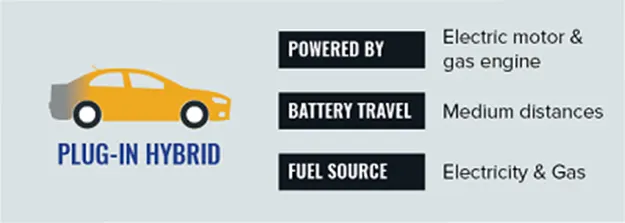
Fig 03. Plug in Hybrid
A battery-powered car, or Battery Electric Vehicle (BEV), does not have a gasoline or diesel engine and instead has an electric motor, power electronics, and a battery pack. Battery cars have a longer all-electric range than a plug-in hybrid, but they do not have a fuel backup. Just like a plug-in hybrid, battery-powered cars plug into an electric outlet to refuel.
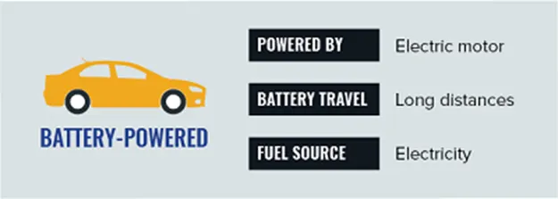
Fig 04. Battery Powered
3.2 Conventional/ Internal Combustion Engines
An internal combustion engine is classified as a heat engine. It’s called internal because the combustion of the air-fuel mixture occurs inside the engine, in a combustion chamber, and some of the burned gases are part of the new combustion cycle.
Basically, an internal combustion engine transforms the thermal energy of the burning air-fuel mixture into mechanical energy. It is called 4 strokes because it takes 4 strokes for the piston to execute a complete combustion cycle. The complete name for an engine which powers a passenger car is: 4 stroke piston internal combustion engines, abbreviated ICE (Internal Combustion Engine).
The cylinder head (8) usually contains the camshaft(s), valves, valve buckets, valve return springs, spark/glow plugs and injectors (for direct injection engines). Through the cylinder head flows the cooling liquid of the engine.
Inside the engine block (12) we can find the piston, connecting rod and crankshaft. As for the cylinder head, through the engine block flows coolant to help control the temperature of the engine.
The piston moves inside the cylinder from BDC to TDC. The combustion chamber is the volume created between piston, cylinder head and engine block when the piston is close to TDC.
In Figure 1 we can examine the complete set of mechanical components of an ICE. Some of the components are fixed (e.g. cylinder head, cylinder block) and some of them are moving. In the figure below we’ll have a look at the main moving part of an ICE, which transform the gas pressure within the cylinder in mechanical power.
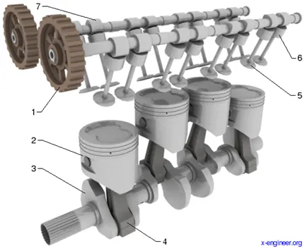
Fig 05. Parts of IC Engines
The rotation of the camshaft is synchronised with the rotation of the crankshaft through a toothed belt or chain. The position of the intake and exhaust valves must be precisely synchronised with the position of the piston, to allow the combustion cycles to take place accordingly.
A complete engine cycle for a 4 stroke ICE has the following phases (strokes):
- intake
- compression
- power (expansion)
- exhaust
A stroke is the movement of the piston between the two dead centres (bottom and top).
Now, that we know which are the components of an ICE, we can examine what is happening in each stroke of the engine cycle. In the table below you’ll see the position of the piston at the beginning of each stroke and the details regarding the events that take place in the cylinder.
Stroke 1 – INTAKE
|
|
At the beginning of the intake stroke the piston is close to TDC. The intake valve is opened, the piston starts to move towards the BDC. Air (or air-fuel mixture) is drawn into the cylinder. This stroke is called INTAKE because fresh air/mixture is taken into the engine. The intake stroke ends when the piston is at the BDC. During the intake stroke, the engine consumes energy (the crankshaft is rotating due to the inertia of the components). |
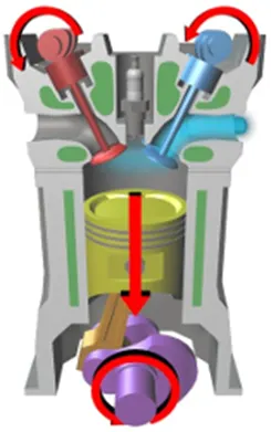 Internal combustion engine intake stroke
Stroke 2 – COMPRESSION
|
|
The compression stroke starts with the piston at BDC, after the intake stroke is finished. During the compression stroke both valves, intake and exhaust, are closed, and the pistons moves towards TDC. With both valves closed, the air/mixture is compressed, reaching maximum pressure when the piston is close to TDC. Before the piston reaches the TDC (but very close to it), during the compression stroke: § for gasoline engine: the spark is generated § for diesel engines: fuel is injected During the compression stroke, the engine consumes energy (the crankshaft is rotating due to the inertia of the components), more than the intake stroke. |
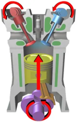 Internal combustion engine compression stroke
Stroke 3 – POWER
|
|
The power stroke starts with the piston at TDC. Both valves, intake and exhaust, are still closed. The air-fuel mixture combustion started at the end of the compression stroke, which causes a significant increase of pressure inside the cylinder. The pressure inside the cylinder pushes the piston down, towards the BDC. Only during the power stroke the engine produces energy. |
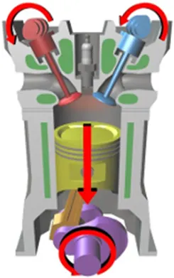 Internal combustion engine power stroke
Stroke 4 – EXHAUST
|
|
The exhaust stroke starts with the piston at the BDC, after the power stroke finished. During this stroke, the exhaust valve is open. The movement of the piston from the BDC towards the TDC pushes most of the exhaust gases out of the cylinder, into the exhaust pipes. During the exhaust stroke, the engine consumes energy (the crankshaft is rotating due to the inertia of the components). |
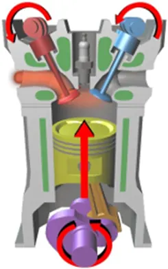 Internal combustion engine exhaust stroke
As we can see, in order to have a complete combustion (engine) cycle the piston has to perform 4 strokes. This means that one engine cycles takes two complete rotations of the crankshaft (720°).
The only stroke which produces torque (energy) is the power stroke, all the others are consuming energy.
|
4 |
Exhaust |
BDC |
Closed |
Open |
Consumes |
For a better understanding, we’re summarising the piston initial position, valve position and energy balance for each stroke.
Table 01. IC Engine stroke cycle
3.3 Forward based conventional vehicle model
The forward modelling approach is also known as cause-effect, engine to wheel or rear to front method. The direction of calculation is same as the direction of positive power flow, i.e., from engine to wheels. This approach is based on vehicle dynamics equations and the behaviour of each powertrain components and their dynamic interactions.
Moreover, a driver controller is required to control the vehicle to follow a desired speed and set the start of controller.
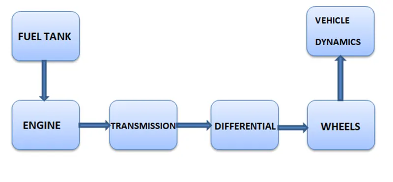
Fig 06. Forward based modelling
A Conventional vehicle body contains internal combustion engine which intake fuel as chemical energy input and converts chemical energy into mechanical energy. The engine output is fed into transmission system where we use gears to transmit power to axle according to driving and road conditions. Axle is connected to gearbox and it transfer power from gear box to differential from where power is transmitted to wheels.
04. Formula used for computation and modelling
Formula for calculating traction forces,
Aerodynamic drag acting on the vehicle
F_ad=1/2*ρ*A*C_d*V²
Where ρ is Density of air
A is Frontal area
C_d is Drag Coefficient
V is Velocity of vehicle
Rolling resistance force
F_rr=C_r*M*g*cosθ
Where C_r is a rolling coefficient
M is mass
Θ is slope angle
Grade Force
F_g=M*g*sinθ
Speed Ratio
SP=Ꙍt/Ꙍp
Where Ꙍt is turbine speed
Ꙍp is pump speed
Torque Ratio
TR=Tt/Tp
Where Tt is turbine torque
Tp is pump torque
Capacity Factor
Kf=Ꙍp/√Tp
Mass Fuel Rate consumption
Mf=Pe/(ⴄe*Q_LHV)
Where Pe is engine power
ⴄe engine efficiency
Q_LHV is low heat value of fuel
Relation between Ring gear, Sun gear and Carrier gear
Ꙍc*(Ns+Nr) = Ꙍs*Ns+Ꙍr*Nr
-Tc/(Ns+Nr)=Ts/Ns=Tr/Nr
Where c s and r represents carrier, sun and ring gear
Ꙍ is the speed
T is the torque
05. Project Overview
5.1 Matlab prerequisites for modelling
We have matlab code to run which stores the variables and the data required to model vehicle block in Simulink. Also we load different drive cycles into matlab workspace and selecting the required drive cycles e can compute the simulink results as per requirement.
We have different state variables require while modelling vehicle body in simulink. We use different data like vehicle parameters, transmission parameters and driver parameters.
The vehicle parameters includes aerodynamic constants like density of air, frontal area, drag coefficient and drag constants like rolling coefficient gravity acceleration etc.
Also transmission coefficients like transmission efficiency, number of gears differential efficiency and final drive ratio.
Different cycle data like UDDS, HWFET, NEDS, FTP, US06 and WLTP are loaded into matlab workspace and we can choose the drive cycle number to perform the simulink model for the respective cycle and analyse the results.
5.2 Matlab Pre-processing Code:
%%%%%%%%%%%%%%%%%%%%%%%%%%%%%%%%%%%%%%%%%%%%%%%%%%%%%%%%%%%%%%%%%%%%%
%% Skill-Lync -> Hybrid Drives Development
% Project 1 - Conventional Vehicle Model
% By - Shivakumar G R

% Description:

%% Initialization File
% Initialization file for loading the variables for the Conventional vehicle simulation model

%% Vehicle Parameters
M = 1500;       % Vehicle weight [kg]
Cr = 0.015;     % Rolling resistance coefficient
Rw = 0.35;      % Rolling radius [m]
Cd = 0.33;      % Drag coefficient
Af = 2;         % Frontal area [m2]
rhoa = 1.225;   % Air density [kg/m3]
Vwind = 0;      % Wind velocity [kmph]
g = 9.81;       % Gravitational acceleration [m/s2]
theta = 0;      % Slope [deg]
myu_road_tire = 1; % Coefficient of friction between tire - road interface

%% Powertrain Parameters
FDR = 3.73;                         % Final Drive Ratio / Diff Ratio
DiffEff = 0.99;                     % Differential efficiency (assumed independent of operating conditions)

NumGear = 4;                        % Number of gears in transmission
TransGear = [1:NumGear];            % Transmission Gears
TransRatio = [3.06, 1.62, 1, 0.7];  % Corresponding Transmission ratios
TransEff = 0.90;                    % Transmission efficiency (assumed independent of operating conditions)

TC_SR = [0, .5, .6, .7, .8, .87, .92, .94, .96, .97, 1];   % Torque Converter Speed Ratio (Matlab default) -> TurbSpd/PumpSpd
TC_TR = [2.232, 1.5462, 1.4058, 1.2746, 1.1528, 1.0732, 1.0192, 1, 1, 1, 1];   % Torque Converter Torque Ratio (Matlab default) -> TurbTrq/PumpTrq
TC_Cf = 1e-4 * [.72558, .66322, .63463, .59042, .51331, .4144, .29287, .22444, .12186, .04386, 0]; % Torque Converter Capacity Factor (Matlab default) -> PumpTrq/PumpSpd^2 [Nm/rpm^2]

load Vehicle_Data/Engine_data_1_9L_Saturn_95kW
load Vehicle_Data/Trans_Shift_map

%% Driver Parameters
Kp = 10;                    % P gain for driver PI model
Ki = 1;                     % I gain for driver PI model
Drive_Cycle_Select = 2;     % Drive cycle selection

% Drive cycle values in m/s

if Drive_Cycle_Select == 1
    load DriveCycles/UDDS;

elseif Drive_Cycle_Select == 2
    load DriveCycles/HWFET;

elseif Drive_Cycle_Select == 3
    load DriveCycles/FTP;

elseif Drive_Cycle_Select == 4
    load DriveCycles/US06;

elseif Drive_Cycle_Select == 5
    load DriveCycles/NEDC;

elseif Drive_Cycle_Select == 6
    load DriveCycles/WLTP;

end

time_end = cyc_time(end);
vel_end = cyc_vel(end);
5.3 Simulink Model
We have our simulink model which has been made multiple subsystems to break the complex system into simpler module. The basic structure of vehicle body looks like,
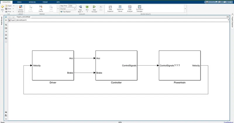
Fig 07. Forward model of a conventional vehicle
The main vehicle body system consist a driver, controller and powertrain block, the driver inputs the acceleration and braking based on the driver input controller unit decides the input variables for the power train like throttle engine torque, brake torque and gear commands required for the powertrain unit.
The power train unit has a multiple subsystem like engine, transmission, differential, wheels and vehicle dynamics. We will be discussing each block in details in coming pages.
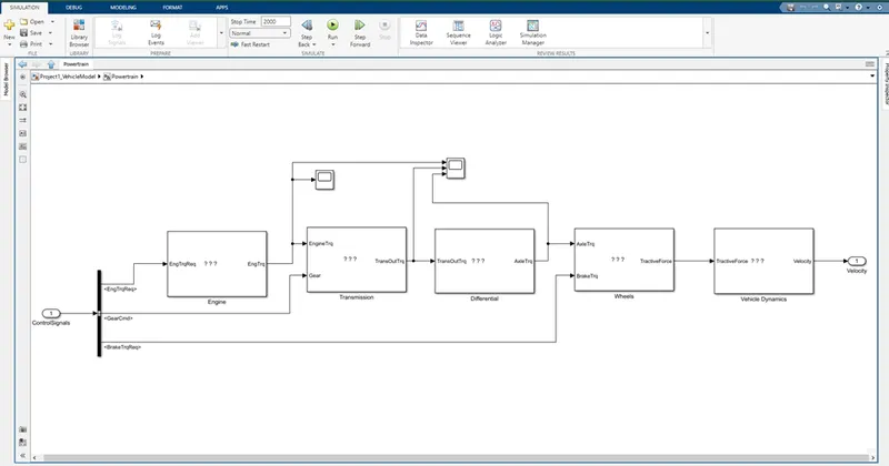
Fig 08. Simulink model of a powertrain subsystem
5.3.1 Driver Subsystem
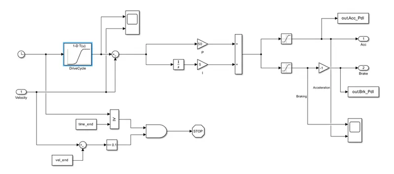
Fig 09. Simulink model of a Driver system
The above blocks represents the driver unit which takes time and speed of the vehicle as input and provides required acceleration and brake as output. We have two conditions to process in the unit during normal driving conditions there will be continuous acceleration brake out accordingly after a while once it reaches end as time and velocity reaches end point the simulation will stop.
The velocity provided integrated and added to provide the final acceleration required. Same way brake is obtained. Both braking and acceleration are segregated using saturation block with positive and negative signals.
5.3.2 Controller Subsystem
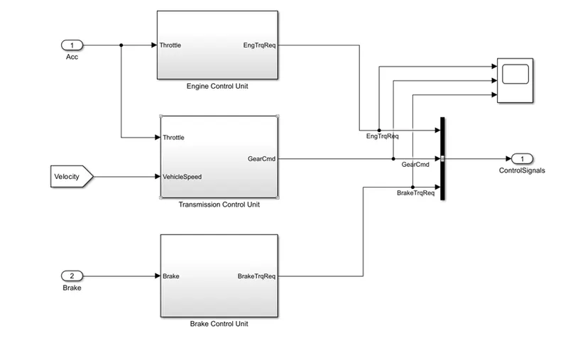
Fig 10. Simulink model of a control system
Control unit takes acceleration and brake as input to provide required torque for engine and braking torque to wheels. Also the control unit provides gear command for the transmission unit.
The controller unit is divided into three more subsystem like engine control unit to provide engine torque transmission control unit which decides the gear command and braking control unit which provides brake torque for the wheels.
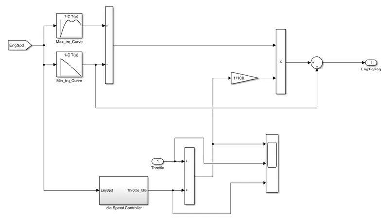
Fig 11. Simulink model of a Engine control unit
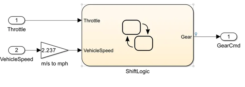
Fig 12. Simulink model of a Transmission control Unit
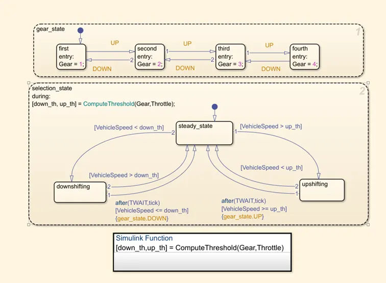
Fig 13. State flow diagram of Shift Logic state flow unit
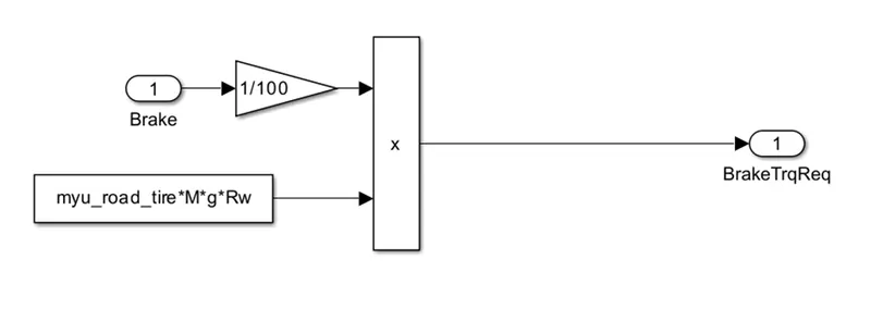
Fig14. Brake Control Unit
All the above images show the subsystem units of controller unit. Engine control unit takes engine speed as input and using 1 D lookup table we compute the torque requirement at each point of speed. Also we can observe the idle speed calculation and engine torque requirement is a product of maximum torque requirement and idle torque. The engine torque required is out of the block and will be a input for engine.
Transmission unit is used to decide the gears and based on which engine speed and torque are achieved at different gear ratios. We use state flow function to calculate the gear command. We can see the shift logic is explained in the above images and gear command is generated.
5.3.3 Engine
Engine is a power train unit block. Engine is called heart of the vehicle system and it is one which converts chemical energy stored in fuel into mechanical energy burning the fuel.
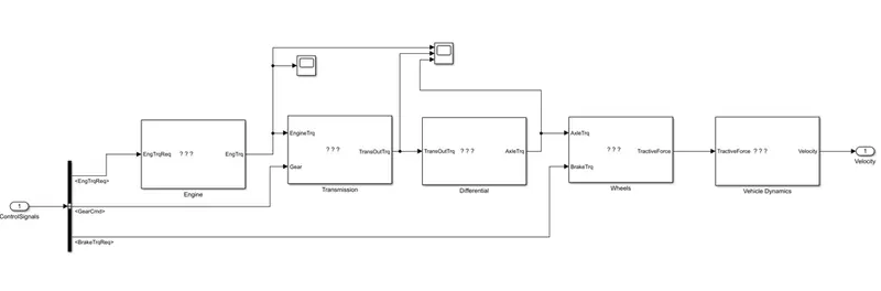
Fig 15. Simulink model of a powertrain
The above image represents the powertrain unit which consist of engine, transmission, differential, Wheels and Vehicle Dynamics blocks. We will be discussing each unit one by one in detail.
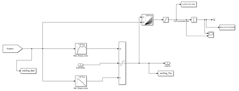
Fig 16. Simulink model of a engine
5.3.4 Transmission
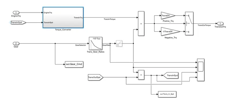
Fig 17. Simulink model of a transmission
The transmission block takes engine torque as input and received by torque converter we get transmission input torque from it also we use the gear command to compute the required gear ratio and product of torque input and gear ration gives us output torque from transmission.
We have 1 D lookup table which takes the gear command and provides the corresponding gear ratio and torque output is multiplied with transmission efficiency to get accurate results.
5.3.5 Differential
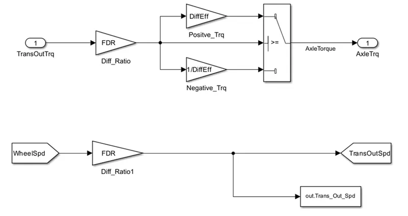
Fig 18. Simulink model of a differential
The transmission output torque is given as input to the differential system and this is multiplied by final drive ratio and differential efficiency to compute axle torque which is given to wheels for the traction.
5.3.6 Wheels
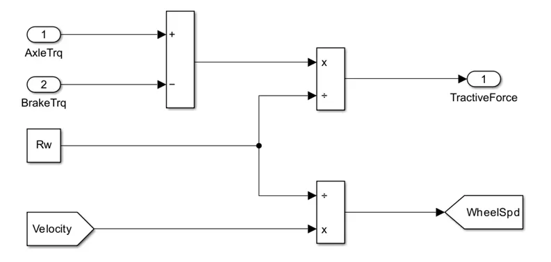
Fig 19. Simulink model of a wheels
Wheels take axle torque and brake as input which is used to compute the tractive forces.
5.3.7 Vehicle Dynamics
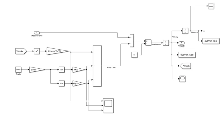
Fig 20. Simulink model of a vehicle Dynamics
A vehicle dynamics unit compute the required traction forces for the vehicle movement. There are different forces acting on the vehicle and all are calculated and added to calculate the final drive force, velocity and distance travelled.
The different types of traction forces acting are,
- Aerodynamic forces
- Rolling resistance
- Grade forces
All the forces are computed and divide by acceleration to calculate the velocity. Velocity is integrated at each time level to calculate the distance travelled.
At level of subsystem we have used scope to record the individual data and its variations. The same data has been imported back into workspace using to workspace block post processing purpose in matlab.
5.4. Post processing Matlab Code:
Once after the simulink model is run we have taken data into workspace and we need to plot the graph for different variables obtained after calculation in order to study the behaviour of vehicle at different conditions.
We take the results to plot for UDDS and HWFET drive cycles.
Post Processing Code:
%%%%%%%%%%%%%%%%%%%%%%%%%%%%%%%%%%%%%%%%%%%%%%%%%%%%%%%%%%%%%%%%%%%%%
%% Skill-Lync -> Hybrid Drives Development
% Project 1 - Conventional Vehicle Model
% By - Shivakumar G R
clc
% Description:
% The following file is to used with the Initialization file and Simulink
% results for post-processing of the data.
% The file is incomplete, has some examples of how the data is imported
% into a readable format, data analysis and plotting examples.
% Based on the project task, use commands in a similar format as given
% below, to analyse the data and generate required plots.
% You can change variable names if desired

%% Post-Processing File
%  File for post-processing the Conventional vehicle simulation model data

%% Renaming variables
Time = out.tout;
Acc_Pdl = out.Acc_Pdl;          % Accelerator pedal [%]
Brk_Pdl = out.Brk_Pdl;          % Brake pedal [%]
Gear_Cmd = out.Gear_Cmd;        % Transmission gear
Trans_In_Spd = out.Trans_In_Spd*30/pi;  % Transmission input speed [rpm]
Trans_Out_Spd = out.Trans_Out_Spd*30/pi;% Transmission output speed [rpm]
Eng_Trq = out.Eng_Trq;          % Engine brake torque [Nm]
Eng_Spd = out.Eng_Spd*30/pi;    % Engine speed [rpm]
Eng_Fuel_Consump = out.Eng_Fuel_Consumption;    % Engine fuel consumption [g]
Veh_Dist = out.Veh_Dist/1000;   % Distance traveled by vehicle [km]
Veh_Spd = out.Veh_Spd*18/5;     % Vehicle speed [kmph]


%% Data Analysis
Eng_Pwr = Eng_Spd*pi/30*Eng_Trq/1000;   % Engine brake power [kW]
rho_petrol = 0.7197;                    % Density of petrol [kg/L]
kmpl = Veh_Dist(end)/(Eng_Fuel_Consump(end)/1000/rho_petrol);    % Fuel economy [kmpl]


%% Plotting vehicle characteristics time trace
figure()
subplot(3,1,1)
hold on
grid on
plot(Time, Acc_Pdl, 'linewidth', 1, 'Color', 'black');
plot(Time, Brk_Pdl, 'linewidth', 1, 'Color', 'red');
ylabel('Pedal [%]')
xlim([0, Time(end)]);
legend('Accel','Brake');
subplot(3,1,2)
hold on
grid on
plot(Time, Trans_In_Spd, 'linewidth', 1, 'Color', 'black');
plot(Time, Trans_Out_Spd, 'linewidth', 1, 'Color', 'red');
ylabel('Speed [rpm]')
xlim([0, Time(end)]);
ylim([0, 6000]);
legend('Trans Input','Trans Output');
subplot(3,1,3)
hold on
grid on
plot(Time, Gear_Cmd, 'linewidth', 1, 'Color', 'black');
xlim([0, Time(end)]);
xlabel('Time [s]');
ylabel('Gear');

%% Plotting engine operating points on engine fuel map
figure('Name','Engine Operating Points');
hold on
grid on
title('Engine Operating Points','fontsize',12);
p1=plot(Eng_map_spd*30/pi,Eng_max_trq,'linewidth',2,'color','r');
p2=line([Eng_map_spd(end)*30/pi Eng_map_spd(end)*30/pi],[0 Eng_max_trq(end)]);
set(p2,'linewidth',2,'linestyle','--','color','b');
p3=line([Eng_map_spd(1)*30/pi Eng_map_spd(1)*30/pi],[0 Eng_max_trq(1)]);
set(p3,'linewidth',2,'linestyle','--','color','b');
[c,h] = contour(Eng_map_spd'*30/pi,Eng_map_trq,Eng_fuel_map');
clabel(c,h);
xlabel('Engine Speed [rpm]');
ylabel('Engine Torque [Nm]');
title('Engine Fuel Consumption Map [g/s]');
legend([p1 p3],{'Max Curve','Operating Points'},'Location','southwest');
axis([Eng_map_spd(1)*30/pi Eng_map_spd(end)*30/pi 0 Eng_map_trq(end)]);

% Display the Fuel Economy Numbers
avg_kmpl=mean(kmpl);
fprintf('The Fuel Consumption rate is:%.2f kmpl\n',avg_kmpl)
06.Results
We will be discussing results obtained from simulink and matlab for both UDDS and HWFET Drive cycles one by one.
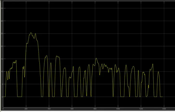
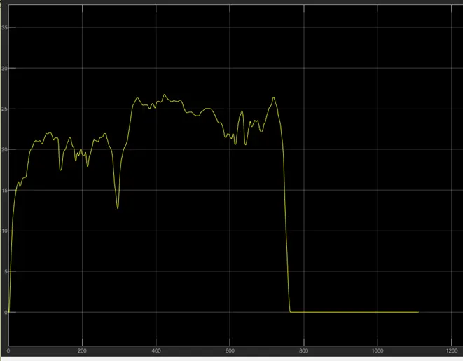
Velocity time graph
UDDS:
HWFET:
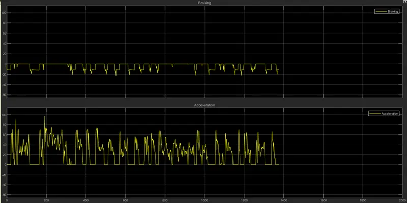
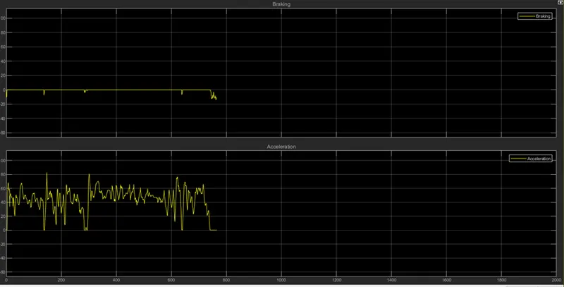
Acceleration and Braking:
UDDS:
HWFET:
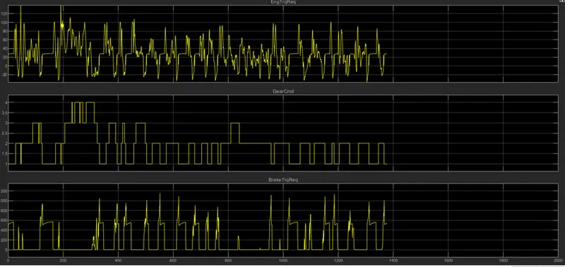
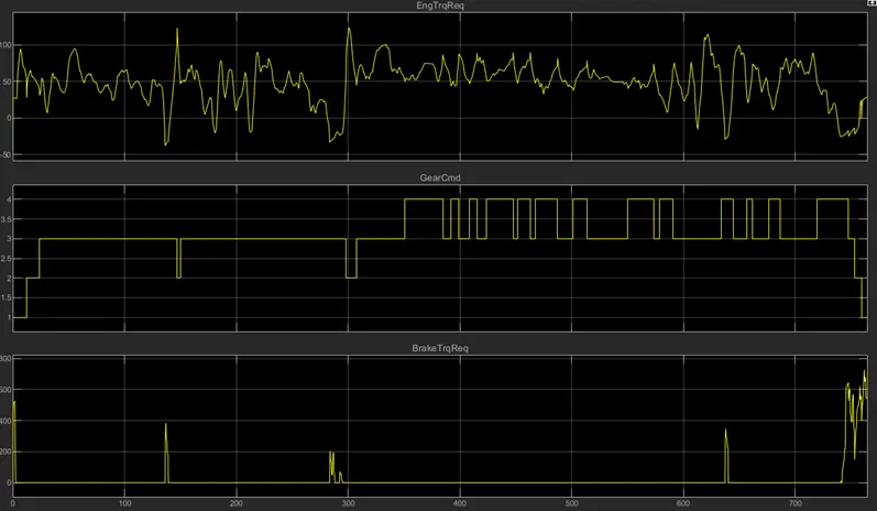
Engine, Brake and Gear command from control unit
UDDS:
HWFET:
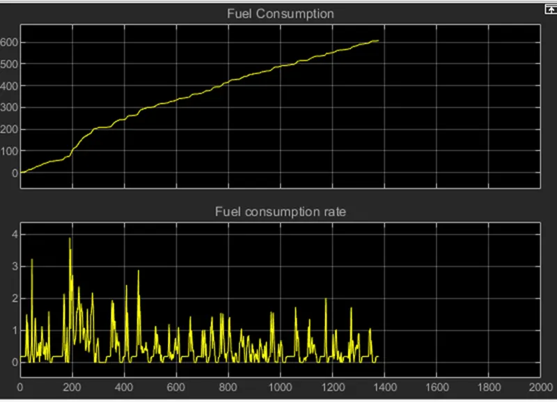
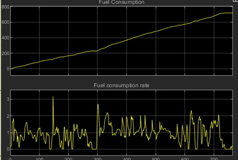
Fuel Consumption Rate and Total Fuel Consumption
UDDS:
HWFET:
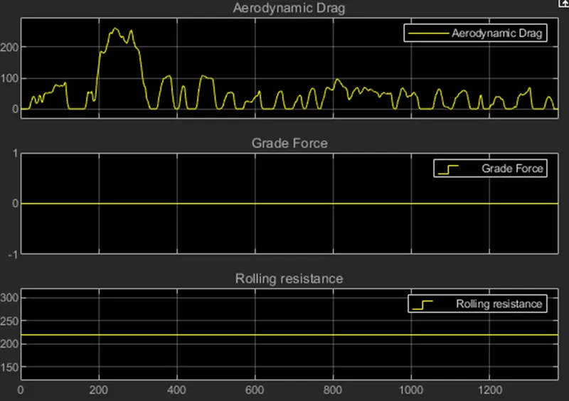
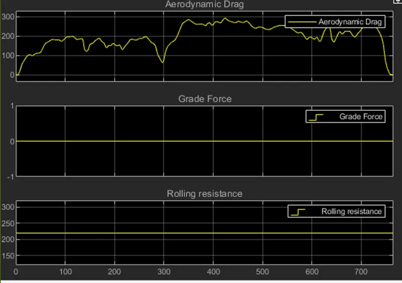
Tractive forces (aerodynamic, grade force and rolling resistance)
UDDS:
HWFET:
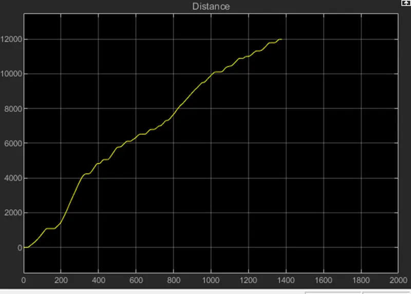
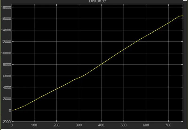
Distance covered with specified time interval
UDDS:
HWFET:
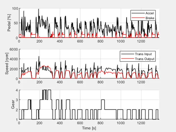
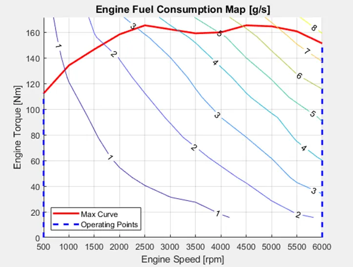
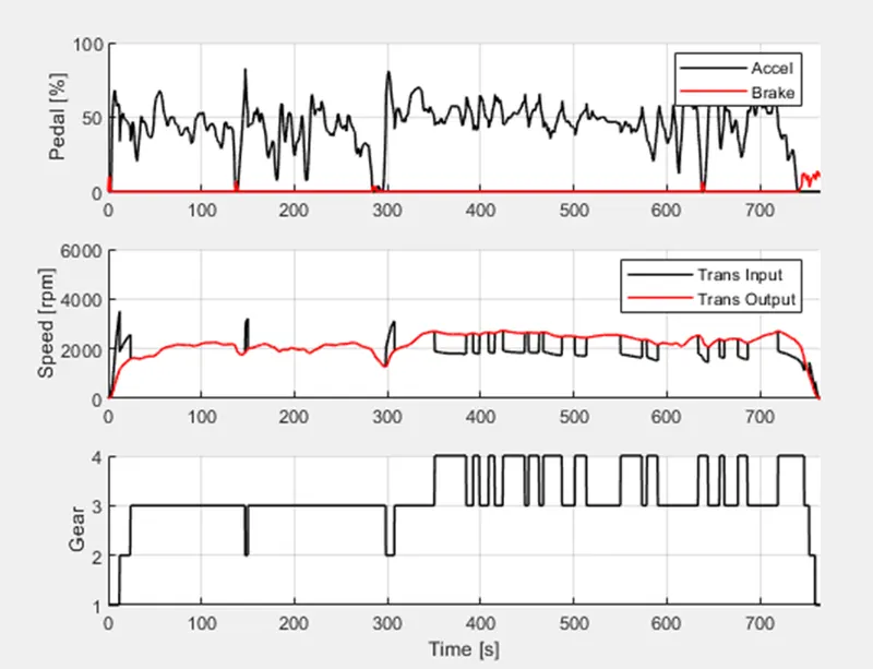
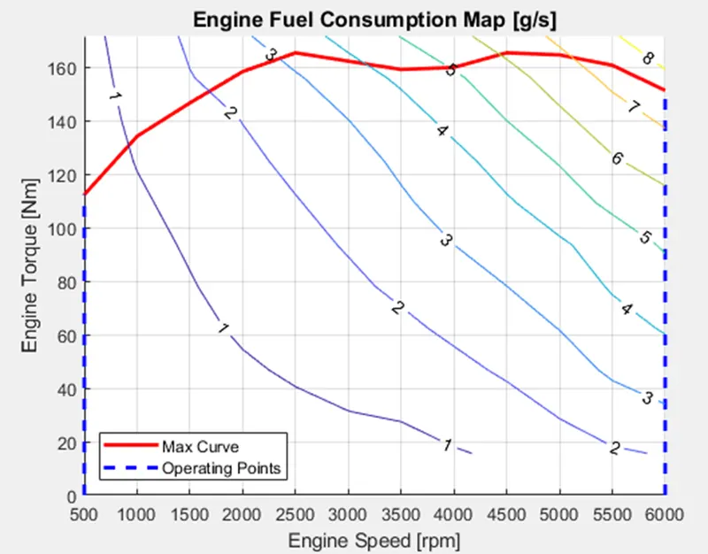
Post processing Matlab Results Obtained:
UDDS:
HWFET:
07. Conclusion:
- We have obtained the graphs for both UDDS and HWFET drive cycles and images are saved.
- Observing velocity curve we can see a lot variation in velocity curve for UDDS cycle where as it is almost maintaining mean value in HWFET. So we can see very less brakes applied here where average acceleration is maintained.
- For UDDS cycle we can observe change of gear command within a short time interval where it is less in Highway cycle. Also Change of Gear s happening for higher velocity control in highway cycle, where for urban drive gear shifting is achieving for maintain lower speed.
- Fuel consumption rate is high for urban drive and where as it is maintained nominal in case of highway drive due to constant velocity and less braking. Overall fuel consumption for urban drive is more for covering shorter distance due to deceleration and braking.
- We have obtained traction forces and can see the variation of aerodynamic drag. The grade is zero as the theta value is zero. The total distance covered in highway cycle is almost linear due to constant speed drive.
- The engine operating points are plotted on the fuel map and the operating point is under the maximum torque curve.
- Using matlab postprocessing code we have plotted graph for acceleration pedal and braking, speed and gear shift for both th drive cycles and maximum operating points are obtained. we can observe that area under maximum operating curve is the power for respective drive cycle.
The fuel Consumption rate for both the cycles is calculated.
UDDS:
The Fuel Consumption rate is:13.26 kmpl
HWFET:
The Fuel Consumption rate is:15.04 kmpl
The drive link for the complete project is attached
https://drive.google.com/drive/folders/1JnVRdUpYUzxk6saPGwurRpJ4jDvegioG?usp=share_link
The detailed project report is uploaded in the pdf format.
08. References:
- https://www.intechopen.com/chapters/19452
- https://www.nyserda.ny.gov/All-Programs/Drive-Clean-Rebate-For-Electric-Cars-Program/About-Electric-Cars/Types-of-Cars#:~:text=Conventional%20vehicles%20use%20an%20internal,used%20to%20move%20the%20vehicle.
- https://x-engineer.org/internal-combustion-engine/
- https://in.mathworks.com/help/autoblks/ug/explore-the-conventional-vehicle-reference-application.html