Plotting of the PV Diagram of an Otto Cycle using MATLAB
Week-2 Report.
- Aim: To write a code that will plot the Pressure vs Volume Graph and then calculate the overall Thermal Efficiency of the Cycle.
- Introduction:
An Otto cycle is an idealized thermodynamic cycle that describes the functioning of a typical spark ignition engine. It is the thermodynamic cycle most commonly found in automobile engines.
The Otto cycle is a description of what happens to a mass of gas as it is subjected to changes of pressure, temperature, volume, addition of heat, and removal of heat. The mass of gas that is subjected to those changes is called the system. The system, in this case, is defined to be the fluid (gas) within the cylinder. By describing the changes that take place within the system, it will also describe in inverse, the system's effect on the environment. In the case of the Otto cycle, the effect will be to produce enough net work from the system so as to propel an automobile and its occupants in the environment.
The Otto cycle is constructed from:
- Top and bottom of the loop: a pair of quasi-parallel and isentropic processes (frictionless, adiabatic reversible).
- Left and right sides of the loop: a pair of parallel isochoric processes (constant volume).
The isentropic process of compression or expansion implies that there will be no inefficiency (loss of mechanical energy), and there be no transfer of heat into or out of the system during that process. The cylinder and piston are assumed to be impermeable to heat during that time. Work is performed on the system during the lower isentropic compression process. Heat flows into the Otto cycle through the left pressurizing process and some of it flows back out through the right depressurizing process. The summation of the work added to the system plus the heat added minus the heat removed yields the net mechanical work generated by the system. A Pressure vs Volume Diagram is shown below:
The Entire Otto cycle can be explained as the following: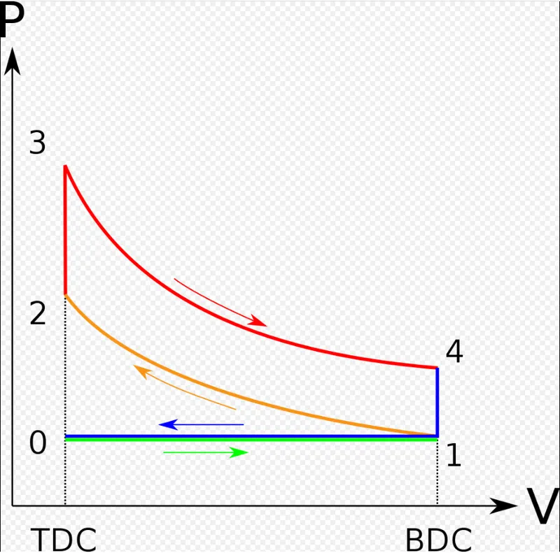
Typical PV Diagram of an Otto Cycle.
- Process 0–1 a mass of air is drawn into piston/cylinder arrangement at constant pressure.
- Process 1–2 is an adiabatic (isentropic) compression of the charge as the piston moves from bottom dead center (BDC) to top dead center (TDC).
- Process 2–3 is a constant-volume heat transfer to the working gas from an external source while the piston is at top dead center. This process is intended to represent the ignition of the fuel-air mixture and the subsequent rapid burning.
- Process 3–4 is an adiabatic (isentropic) expansion (power stroke).
- Process 4–1 completes the cycle by a constant-volume process in which heat is rejected from the air while the piston is at bottom dead center.
- Process 1–0 the mass of air is released to the atmosphere in a constant pressure process.
The Otto cycle consists of isentropic compression, heat addition at constant volume, isentropic expansion, and rejection of heat at constant volume. In the case of a four-stroke Otto cycle, technically there are two additional processes: one for the exhaust of waste heat and combustion products at constant pressure (isobaric), and one for the intake of cool oxygen-rich air also at constant pressure; however, these are often omitted in a simplified analysis. Even though those two processes are critical to the functioning of a real engine, wherein the details of heat transfer and combustion chemistry are relevant, for the simplified analysis of the thermodynamic cycle, it is more convenient to assume that all of the waste-heat is removed during a single volume change.
- Code/Logic:
1. 1. We firstly need to clear and close all the previously entered codes and the preset values of the already used variables, hence we use the following commands:
close all
clear all
clc
2. In the next step, we will include all the general basic inputs such as the Specific Heat of the gas being used, which is γ">γγ= 1.4, which is the specific heat for air in general. Another input would be the Temperature at the end of state point3, which would be T3=2000K. We also need to give the initial conditions such as the Pressure and Temperature at state point1. Using these basic inputs, we can further calculate the Pressure, Temperature and Volume at all the state points and then plot the P-V diagram for the same.
3. We need the Basic Engine Kinematics such as the Bore Diameter, Stroke Length, Compression Ratio etc. All the basic engine parameters were then mentioned as follows:
Bore Diameter = 0.1m
Stroke Length = 0.1m
Length of the Connecting Rod= 0.15m
Compression Ratio = 12
4. To start with the plotting and all the calculations, we need to firstly write a code to calculate the Swept Volume and hence the Clearance Volume.
We know:
a. Swept volume = Volume of the Cylinder = π4(B2L)">π4(B2L)π4(B2L) ; Where, B= Bore Diameter and L=Stroke length of the cylinder.
b. Clearance Volume = During the Compression cycle, the volume that the gases occupy at the TDC is known is Clearance Volume = Swept Volume / (Compression Ratio -1)
Now, we know, V1 = Swept Volume + Clearance Volume
and V2 = Clearance Volume
5. Now, as the Process is a Reversible Adiabatic Expansion of the gas, we know that : PVγ">PVγPVγ = Constant.
Like this, we can calculate the Pressure at state point 2, i.e. P2.
6. Next we use the ideal gas law, also called the general gas equation which is the equation of state of a hypothetical ideal gas.
PV = nRT
Here, P= Pressure
V = Volume
n = Amount of Substance
R = Ideal Gas constant
T = Temperature
so, p1v1t1">p1v1t1p1v1t1 = p2v2t2">p2v2t2p2v2t2
Like this, we can calculate the Temperature at the state point 2, i.e. t2.
7. In the next step, we define a function in a new script. We understand that the function is a piece of code that we can reuse by just calling in its name and the passing of the appropriate parameters.
So, we define a function in the name of engine_kinematics. In this function, we will give various inputs, such as the bore, stroke, compression ratio, start crank angle, end crank angle etc. So, after defining this function, we can define the final output as the compression volume. We basically define this function so that we can then call it again in the main code and then use the inputs from the main code to calculate the output of the function. We use a different formula to calculate the Volumetric Efficiency of the engine to understand the volume in a Combustion chamber changes as the combustion progresses.
The function and the Main code are given below.
8. After this, we then calculate the Pressure and the Volume values at the compression and expansion in the cylinder using the formula of
PVγ">PVγPVγ = constant
9. The last step before we plot all the results, we must give the command of Figure(1) so that the software understands that all the plots are to be given under this figure window. We also need to use the Hold on command so that all the plots are drawn one after the other, otherwise all the previous plots will be overwritten instead and we will only get the last plot as a result of the run.
10. The next step is to give all the commands to plot the appropriate co-ordinates and the lines as well. It is shown in the command window below.
11. The last step is to calculate the Thermal Efficiency of the Otto Cycle.
The formula is as follows:
η">ηη = 1 - (1/compression ratio^[γ">γγ-1])
Using this formula, we can calculate the Thermal Efficiency of the Cycle.
The Main Code is as follows:
clear all
close all
clc
%Inputs gamma = 1.4;
t3 = 2000;
%Initial State Variables
p1 = 101325;
t1 = 500;
%Engine Variables
bore = 0.1;
stroke = 0.1;
con_rod = 0.15;
cr = 12;
%Calculating Swept volume
v_swept = (pi/4)*bore^2*stroke;
v_clearance = v_swept / (cr -1);
v1 = v_swept + v_clearance;
v2 = v_clearance;
%State variables at state point 2
%p2v2^gamma = p1v1^gamma
p2 = p1 * cr^gamma
%Using Ideal Gas Law
%p1v1/t` = p2v2/t2
t2 = p2 * v2 * t1 / (p1 * v1);
%Calculating the volume and pressure under Compression
constant_c = p1*v1^gamma;
V_compression = engine_kinematics(bore, stroke , con_rod, cr, 180,0);
p_compression = constant_c./ V_compression.^gamma;
%State variables at state point3 (const volume combustion process)
v3 = v2;
%Using Ideal Gas Law
p3 = p2*t3 / t2;
%Calculating the Volume and Pressure under Expansion
constant_c = p3*v3^gamma;
V_expansion = engine_kinematics(bore, stroke , con_rod, cr, 0, 180);
p_expansion = constant_c./ V_expansion.^gamma;
%State variables at state point4
v4 = v1;
%p3v3^gamma = p4v4^gamma
p4 = p3*(v3/v4)^gamma;
figure (1)
hold on
%Plotting all the Results
plot( v1,p1, '*', 'color', 'r')
plot(V_compression, p_compression)
plot( v2,p2, '*', 'color', 'r')
plot([v1,v4], [p1,p4], 'color', 'r')
plot( v3,p3, '*', 'color', 'r')
plot(V_expansion, p_expansion)
plot(v4,p4, '*', 'color', 'r')
plot([v2,v3], [p2,p3], 'color', 'r')
xlabel ('Volume (m^3)')
ylabel ('Pressure (N/m^2)')
grid on
%Thermal Efficiency of the Otto Cycle
eta = 1 - (1/cr^[gamma-1])
The Function for this is as follows:
%the function
function [V_compression] = engine_kinematics(bore, stroke , con_rod, cr, start_crank, end_crank)
%crankpin radius
a = stroke/2
R= con_rod / a
v_s = (pi/4)*bore^2*stroke
v_c = v_s / (cr -1)
theta = linspace(start_crank,end_crank,100)
%formula use: V/V_c =
%1+(0.5)(r_c-1)[R+1-cosd(theta)-(R^2-sin(theta)^2)^0.5]
term1 = 0.5 * (cr-1)
term2 = R +1 - cosd(theta)
term3 = (R^2 - sind(theta).^2).^(0.5)
V_compression = (1+term1 * (term2 - term3)).* v_c
end
- Results: Before we get the Final graph, we get the State points as follows:
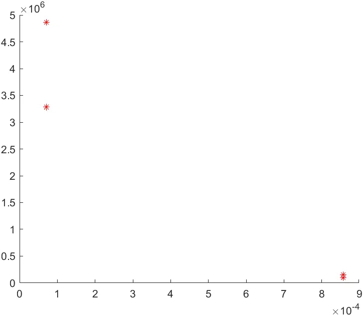
State Points of the PV Diagram.
The Pressure-Volume graph for the Otto cycle is as follows: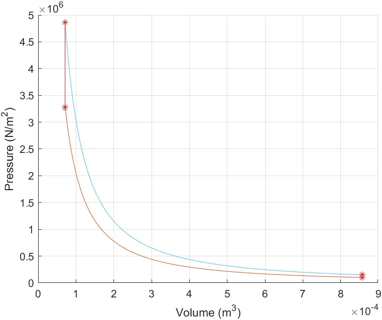
PV Diagram of the otto cycle.
- Errors: The errors that I faced were majorly the typos and the parantheses brackets erros on certain commands. So, when MATLAB pointed out the mistakes, I went to that particular line and corrected the errors.
- Conclusion: In conclusion I would like to state that this challenge helped me understand how to write a code to analyse an Air standard Cycle and the basics of how to use a function in a main code.