PID Controllers

1) In which situations feedforward control of DC motor fails? Prepare a MATLAB script for feedforward control and test it.

DC Motor control design:

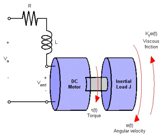
Both electrical and mechanical components are represents here, with the DC motor modelling constants as:

`T=K_mI_a`

`V_(emf)=K_bomega`

The torque T(t) and angular velocity w(t) are what we are interested in

Electrical:

`V_a=I_aR_a+L(di)/dt+V_(emf)`

`V_a-V_(emf)=T/K_m(R_a+Ls)`

`T=K_m/(R_a+Ls)(V_a-V_(emf))`

Mechanical:

`T=J(domega)/dt+T_(load)`

`T=J(domega)/dt+K_fomega`

`T=omega(Js+K_f)`

`omega=T/(Js+K_f)`

Feedforward DC motor control design:

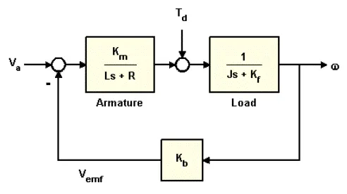
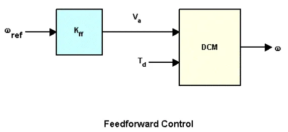
Feedforward control is a method in which the compensator (in this case `K_(ff)`) is the inverse of the transfer function (DCM) so that `omega_(ref) approx omega`

However, since this is not a feedback system, the method only works if the exact disturbance `T_d` and transfer function DCM is known. Without those, simply making `K_(ff)` the inverse of DCM will give poor results.

R = 2.0;                % Ohms
L = 0.5;                % Henrys
Km = 0.1;               % torque constant
Kb = 0.1;               % back emf constant
Kf = 0.2;               % Nms
J = 0.02;               % kg.m^2/s^2

% First construct a state-space model of the DC motor with two inputs
% (Va,Td) and one output (w):

h1 = tf(Km,[L R]);            % armature
h2 = tf(1,[J Kf]);            % eqn of motion

dcm = ss(h2) * [h1 , 1];      % w = h2 * (h1*Va + Td)
dcm = feedback(dcm,Kb,1,1);   % close back emf loop

Feedforward DC Motor Control Design
% You can use this simple feedforward control structure to command 
% the angular velocity w to a given value w_ref. 
%
% <<../dcdemofigures_03.png>>
%
% The feedforward gain Kff should be set to the reciprocal of the DC gain
% from Va to w.
%
Kff = 1/dcgain(dcm(1))

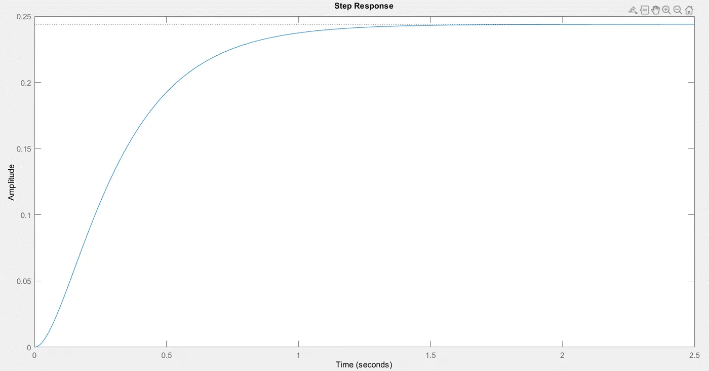
Now plot the angular velocity response to a step change in voltage Va:
%
stepplot(dcm(1));

%%
% To evaluate the feedforward design in the face of load disturbances,
% simulate the response to a step command w_ref=1 with a disturbance Td =
% -0.1Nm  between t=5 and t=10 seconds:
%
t = 0:0.1:15;
Td = -0.1 * (t>5 & t<10);       % load disturbance
u = [ones(size(t)) ; Td];       % w_ref=1 and Td

cl_ff = dcm * diag([Kff,1]);    % add feedforward gain
cl_ff.InputName = {'w_ref','Td'};
cl_ff.OutputName = 'w';

h = lsimplot(cl_ff,u,t);
title('Setpoint tracking and disturbance rejection')
legend('cl\_ff')

% Annotate plot
line([5,5],[.2,.3]); 
line([10,10],[.2,.3]);
text(7.5,.25,{'disturbance','T_d = -0.1Nm'},...
            'vertic','middle','horiz','center','color','r');

Step plot:

Applying feedforward control and disturbance:

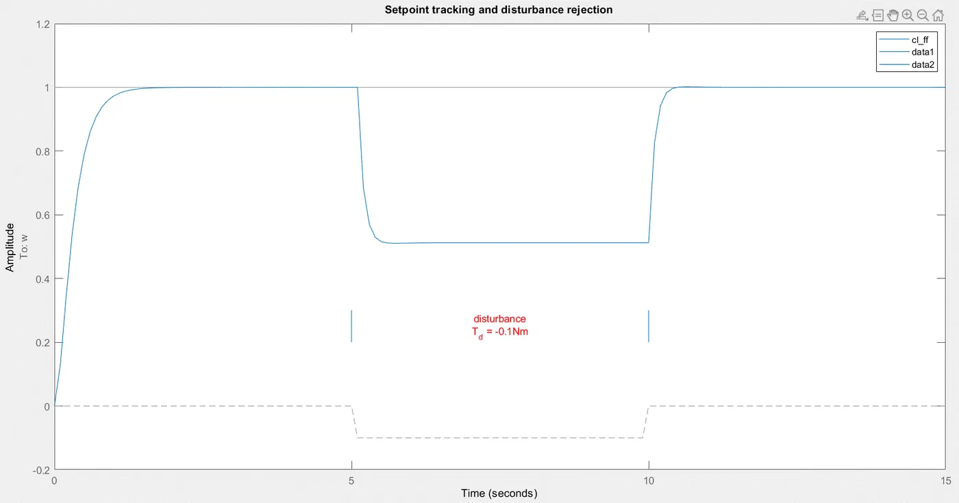
• After applying feedforward control, although all parameters have improved (rise time, steady state error, settling time), the output also shows how poor the response is to disturbance
• Adding a disturbance by applying 0.1Nm of load torque in the opposite direction of the DCM completely changes the step response between 5-10 seconds. The system is unable to reject the disturbance and hence is unstable in that time interval.
• This is a huge limitation to this method. As soon as there appears disturbance that is unaccounted for, the system becomes unstable as there is no sensor to detect the error and adjust the system accordingly using feedback control. Realistically, it will seldom be possible to account for every possible disturbance, and without that this feedforward control method would not be recommended.

2) Assume a plant and controller. Using MATLAB PID controller block verify system response with General Observation for PID gain:

Setup:

Untuned step response:

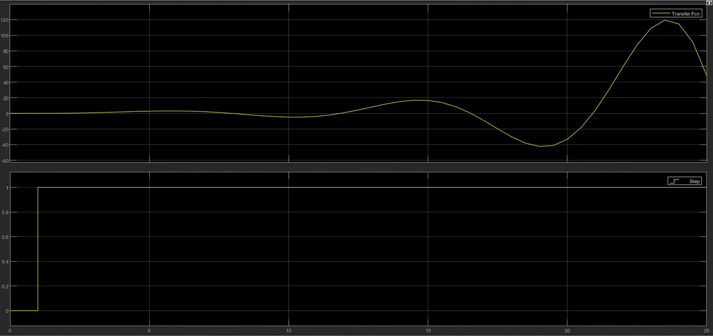
• It is evident that the step response of this function is unstable, as it continues to rise with time.

Testing Kp, Ki, Kd

Kp = 10; Ki = 10; Kd = 5

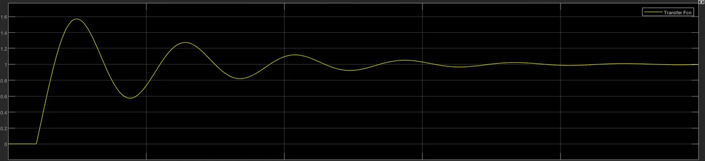
Kp increased; Ki increase; Kd unchanged - Rise time reduced, Overshoot increased, Settling time increased (as both Kp and Ki are incremented), and S-S error reduced

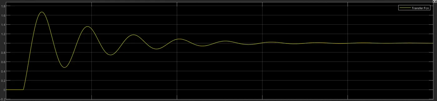
Kp increased; Ki increase; Kd unchanged - Rise time reduced, Overshoot increased, Settling time increased (as both Kp and Ki are incremented), and S-S error reduced

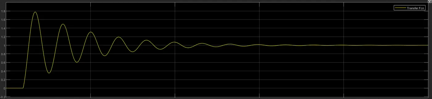
Kp unchanged; Ki unchanged; Kd increased - Minimal change in Rise time, Overshoot reduced, Settling time reduced, Minimal change in S-S error

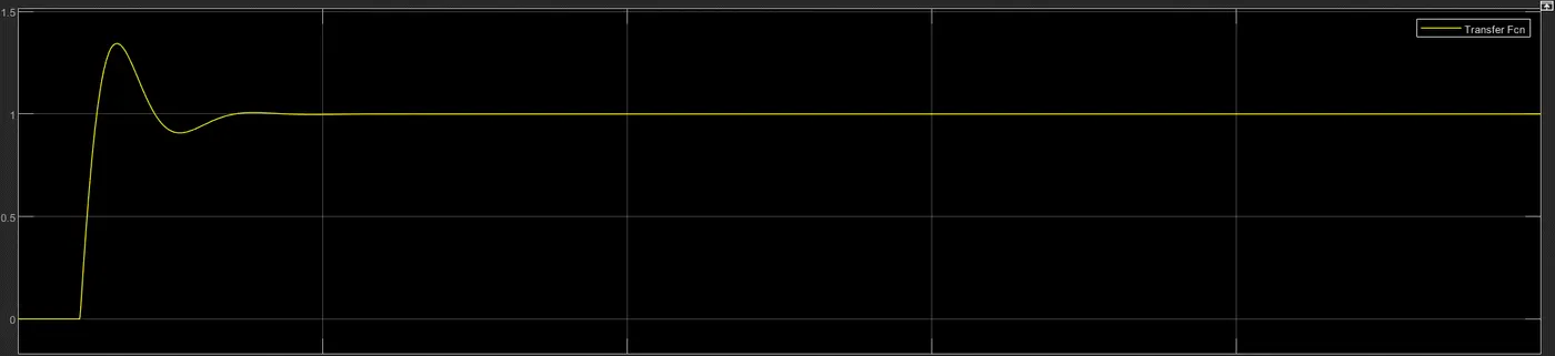
General Observation for PID gain:

Parameters
	Rise time	Overshoot	Settling time	Steady state error
Kp ↑	Decrease	Increase	Small change	Decrease
Ki ↑	Decrease	Increase	Increase	Eliminate
Kd ↑	Small change	Decrease	Decrease	Small change

As expected, the output has responded to the PID controller as per the general observations

3) Use MATLAB PID tuner with the above example and prepare a table showing PID values with response time and transient behaviour coefficient

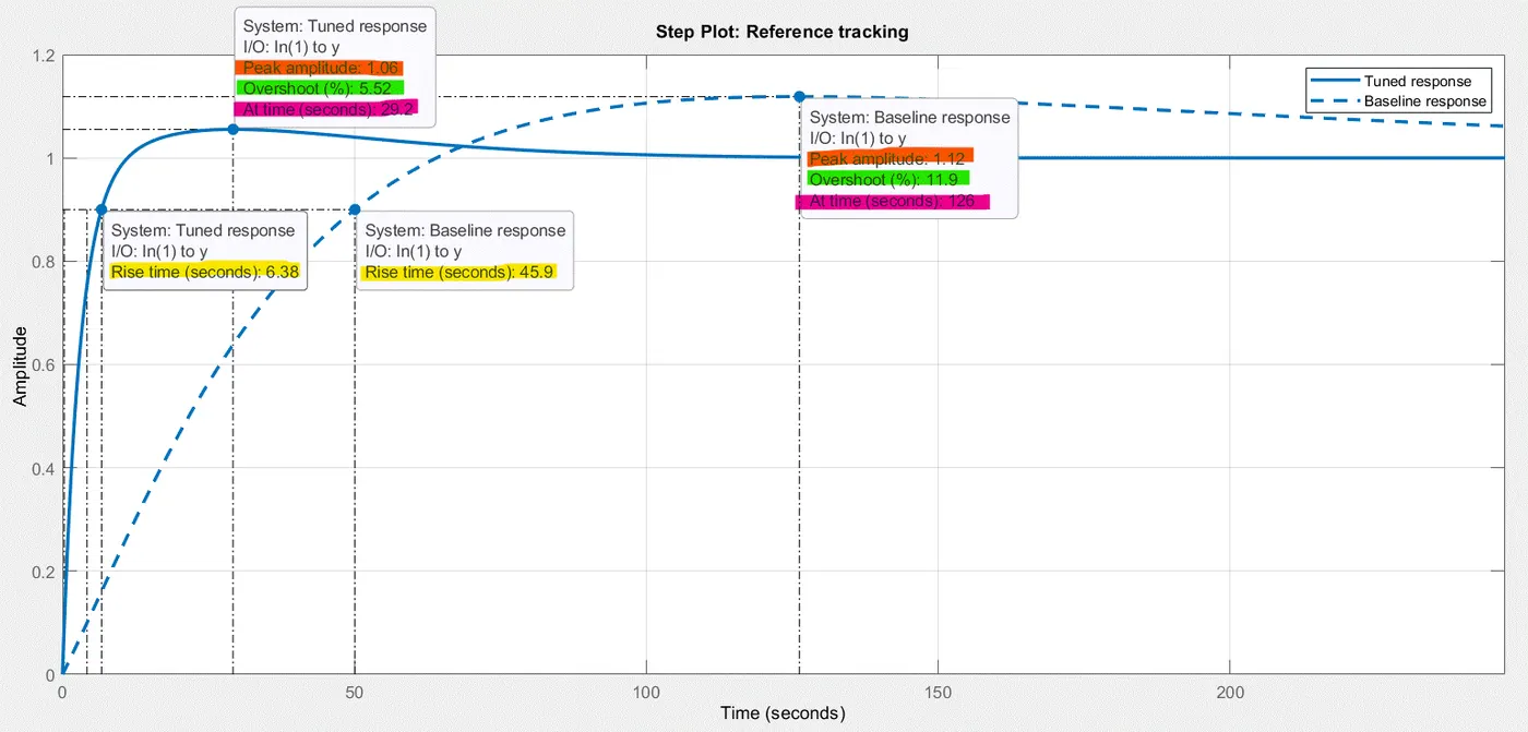
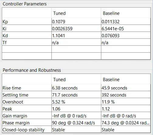
• Using MATLAB PID tuner, it becomes very easy and interactive to explore different options and test to see what gives the desirable results.
• In this example, with a PID tuner, max values of response time and transient behaviour would give best results as is seen.