Solving Second Order ODEs: Simple Pendulum using MATLAB

Aim:

• To construct, solve, and simulate a simple pendulum with damping

Objective:

• Write the code to solve an ODE that represents the motion of a pendulum
• Plot displacement and angular velocity with respect to time
• Create an animation of the simulation

Introduction:

ODEs are used to describe the transient behaviour of engineering systems, and a damped pendulum is an example of such a system.

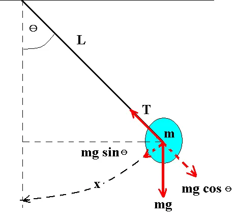
Through balancing forces, the following equation is obtained:

`(d^2theta)/(dt^2)=-g/Lsintheta-b/m(d(theta))/dt` ------------- (`1`)

where:

g = acceleration due to gravity

L = length of string

b = damping coefficient

m = mass of bob

For MATLAB to solve second-order ODEs, equation (1) first needs to be transformed into two first-order ODEs, and then expressed in the form of matrices. The displacement and velocity values with respect to time can then be obtained through the software's inbuilt solver: ode45. Thus, we assume:

• `theta = theta_1` ------------------ (2)

• `(d(theta_1))/dt = theta_2` ----------------- (3)

Hence, equation (1) is transformed into:

`(d(theta_2))/dt = -g/Lsintheta_1-b/mtheta_2` --------------- (`1_(n e w)`)

In terms of a matrix:

`d/dt[[theta_1],[theta_2]]=[[theta_1],[-g/Lsintheta_1-b/mtheta_2]]`

(where obtaining the values of `theta_1` and `theta_2` will represent displacement and velocity, respectively)

MATLAB's inbuilt ODE solver, ode45, performs numerical integration on the set of differential equations that have been represented in the matrix above after taking into account lower and upper bounds of time (`t_0 and t_f`) and initial conditions.

Code for main program:

%solving ODE to model a pendulum

b = 0.05; %damping coeff: kg/s
m = 1; %kg
g = 9.81; %m/s^2
L = 1; %m

%initial condition
theta_0 = [0;3]; %initial displacement = 0 while initial velocity = 3

%time points
t_span = linspace(0,20,500); %taking 500 values between 0-20sec

%solving ODE
[t,results] = ode45(@(t,theta) ode_func(t,theta,b,g,L,m),t_span,theta_0);
figure(1)
plot(t,results(:,1),'linewidth',0.5) %plotting everything in the first column of the results (displacement) with respect to time
hold on
plot(t,results(:,2),'linewidth',0.5) %plotting everything in the second column of the results (velocity) with respect to time
ylabel('plot')
xlabel('time (sec)')
legend('displacement (rad)','angular velocity (rad/sec)')


%animation
figure(2)
changing_theta = results(:,1); %refers to the entire column of theta
num = 1;
for i=1:length(changing_theta)
    angle = changing_theta(i);
   x_initial = 0; %initial coordinates of the pendulum ball
   y_initial = 0;
   x_final = L*sin((pi) - angle); %final coordinates of the pendulum ball
   y_final = L*cos((pi) - angle);
   plot([-5 5],[0 0],'linewidth',2,'color','b'); %base of fixed point
   hold on
   line([x_initial x_final],[y_initial y_final],'linewidth',1,'color','r');
   hold on
   plot(x_final, y_final,'o','markersize',15,'markerfacecolor','r'); %pendulum ball
   axis([-1.5 1.5 -2 0])
   hold off
   pause(0.02)
   M(num) = getframe(gcf);
   num = num + 1;
end

movie(M)
VideoFile = VideoWriter('Simple_Pendulum.avi','Uncompressed AVI');
open(VideoFile)
writeVideo(VideoFile,M)
close(VideoFile)

Code for function:

function [dtheta_dt] = ode_func(t,theta,b,g,L,m)

theta1 = theta(1); 
theta2 = theta(2);

dtheta1_dt = theta2;
dtheta2_dt = -(g/L)*sin(theta1) -(b/m)*theta2;
dtheta_dt = [dtheta1_dt; dtheta2_dt];

end

Output curve:

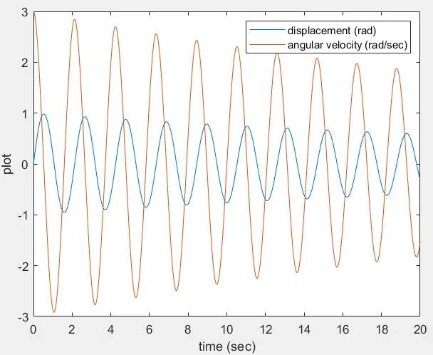
It is evident how the displacement and angular velocity of the bob is affected due to the damper, which is an external force that acts on the system. The higher the damping coefficient, the quicker the motion of the oscillator comes to rest, however due to the low damping coefficient, the motion of the bob will continue much beyond 20 seconds, as is observable from the figure above.

Simulation of the damped pendulum can be viewed through the link below:

https://drive.google.com/file/d/1buO4il_m_xdf7la0RR0GXy1Kw4VJdHUg/view?usp=sharing