Optimizing the Stalagmite function through Genetic Algorithm using MATLAB

Aim:

• Finding the global maxima of the stalagmite function through optimization

Objectives:

• Introduce the concept of genetic algorithm
• Showcasing the process of optimization through three progressive studies
• Plotting graphs to demonstrate the results

Theory:

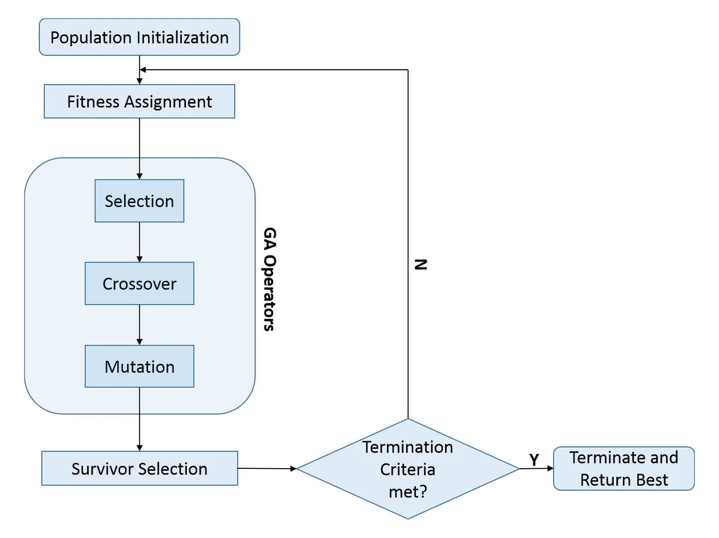
Genetic algorithm is a search-based optimization technique based on the principles of genetics and evolutionary biology, inspired by Charles Darwin's theory of natural evolution. The algorithm reflects the process of natural selection, where the fittest individuals are selected for reproducing the offspring of the next generation. Over successive generations, the population evolves towards an optimal solution.

The entire process is carried out in five phases:

1. Initial population: selection of fittest individuals from a population, where each individual is a potential solution to the problem. Each individual is characterized by a set of parameters (variables) known as genes. Genes join together into a string to form a chromosome (solution). The chromosome is a binary string of 0s and 1s.
2. Fitness function: determines how "fit" each individual is (i.e. the ability to compete with other individuals) by generating a fitness score.
3. Selection: selecting the fittest individuals and allowing them to pass on their genes to the next generation. This process happens in pairs (representing parents)
4. Crossover: For each parent to mate, a crossover point is selected at random from within the genes. Parents exchange genes amongst themselves until the crossover point is reached. The new offspring is then created and added to the population.
5. Mutation: some of the bits in the string can be flipped (0s can becomes 1s and vice-versa). This phases occurs to prevent premature convergence and to maintain diversity. The algorithm terminates if the new offspring produced is not significantly different from the previous generation. This is when convergence is reached and a set of optimal solutions are generated.

*The sequence of phases are repeated to produce individuals in the new generation that are better than the old generation, which is in line with the theory of "Survival of the Fittest".

The algorithm stops when the stopping/termination criteria is met. The algorithm uses the following conditions to determine when to stop:

• Stop after a fixed number of generations
• Stop after a fixed amount of time
• Stop when a chromosome reaches the fitness limit
• Stop when a chromosome succeeds in solving the problem, within a specified tolerance

Genetic algorithm (GA) syntax:

%GA syntax

[coordinates, fval] = ga(fun,nvars) %coordinates represent the x-y coordinates; fval represents the value of the local unconstrained minimum; fun = objective function; nvars = number of variables in the objective function

[coordinates, fval] = ga(fun,nvars,A,b) %linear inequality where A*x is less than or equal to b

[coordinates, fval] = ga(fun,nvars,A,b,Aeq,beq) %linear equality where Aeq*x = beq

[coordinates, fval] = ga(fun,nvars,A,b,Aeq,beq,lb,ub) %lower bound and upper bound respectively

[coordinates, fval] = ga(fun,nvars,A,b,Aeq,beq,lb,ub,nonlcon,Intcon,options) %nonlcon = nonlinear constraints; variables listen in "Intcon" take integer values; replacing default optimization parameter values in "options"

Stalagmite function for which the global maxima needs to be found:

`f_(1x) = [sin(5.1pix+0.5)]^6`

`f_(1y) = [sin(5.1piy+0.5)]^6`

`f_(2x)=e^(-4ln2*((x-0.0667)^2)/(0.64)`

`f_(2y)=e^(-4ln2*((y-0.0667)^2)/(0.64)`

`f(x,y)=f_(1x)*f_(2x)*f_(1y)*f_(2y)`

Stalagmite function code:

function f = stalagmite(input_vector)

xx = input_vector(1);
yy  = input_vector(2);

f1x = (sin(5.1*pi*xx + 0.5))^(6);
f2x = exp((-4*log(2)*(xx-0.0667)^2)/(0.64));

f1y = (sin(5.1*pi*yy + 0.5))^(6);
f2y = exp((-4*log(2)*(yy-0.0667)^2)/(0.64));

f = -(f1x*f2x*f1y*f2y); %multipying the objective function by -1 will give maximum

end

*Optimizing the above function takes place in three progressive studies. The code for the three studies is shown below.

Study 1: Statistical behaviour with unbounded inputs

clear all; close all; clc

x = linspace(-0.5,0.5,200);
y = linspace(-0.5,0.5,200);
num_its = 50;

[xx,yy] = meshgrid(x,y); %creating a 2D array

for i = 1:length(xx) %for every value of x, every value of y will be taken into account
    for j = 1:length(yy)
        input_vector(1) = xx(i,j); %a row vector with 2 columns is created to store the values generated
        input_vector(2) = yy(i,j);      
        f(i,j) = stalagmite(input_vector);
    end
end


%Study 1: the following code is the most generic code for genetic algorithm to
%determine various solutions through random sampling that could potentially be the global maxima

tic
for k = 1:num_its
    [coordinates, fval] = ga(@stalagmite,2);
    xopt(k) = coordinates(1);
    yopt(k) = coordinates(2);
    fopt(k) = -fval;
end

study1_time = toc;

figure(1)
subplot(2,1,1)
hold on
surfc(xx,yy,-f) %multiplying by -1 to plot the actual stalagmite function
shading interp
plot3(xopt,yopt,fopt,'marker','o','markersize',5,'markerfacecolor','k')
title('Statistical behaviour: Unbounded inputs')
xlabel('x-axis')
ylabel('y-axis')
subplot(2,1,2)
plot(fopt)
xlabel('Iterations')
ylabel('Function maximum')

Output 1:

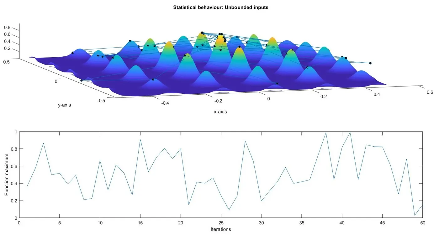
With reference to the code for this study, GA is based on random sampling and the optimum value keeps changing, as is evident in the surface plot and also the graphical plot above. Because all values are randomized and a different answer is generated with every iteration with no scope of convergence, this approach is unusable. Having paid closer attention to the surface plot, it is visible that the solutions generated by GA have gone outside the ideal search region. This is because GA doesn't actually know the bounds it is supposed to search within, leading to many more solutions that are nowhere near the optimum value. This provides the hint to define the lower and upper bounds that the GA is supposed to search within.

Study 2: Statistical behaviour with bounded inputs

clear all; close all; clc

x = linspace(-0.5,0.5,200);
y = linspace(-0.5,0.5,200);
num_its = 50;

[xx,yy] = meshgrid(x,y); %creating a 2D array

for i = 1:length(xx) %for every value of x, every value of y will be taken into account
    for j = 1:length(yy)
        input_vector(1) = xx(i,j); %a row vector with 2 columns is created to store the values generated
        input_vector(2) = yy(i,j);      
        f(i,j) = stalagmite(input_vector);
    end
end

%Study 2: now we need to figure out how to narrow down the search space for the
%algorithm to determine the optimal solution out of all the initial
%solutions it has produced in Study 1

tic
for k = 1:num_its
    [coordinates, fval] = ga(@stalagmite,2,[],[],[],[],[-0.2;-0.2],[0.35;0.35]);
    xopt(k) = coordinates(1);
    yopt(k) = coordinates(2);
    fopt(k) = -fval;
end

study2_time = toc;

figure(2)
subplot(2,1,1)
hold on
surfc(xx,yy,-f) %multiplying by -1 to plot the actual stalagmite function
shading interp
plot3(xopt,yopt,fopt,'marker','o','markersize',5,'markerfacecolor','k')
title('Bounded inputs')
xlabel('x-axis')
ylabel('y-axis')
subplot(2,1,2)
plot(fopt)
xlabel('Iterations')
ylabel('Function maximum')

With reference to the code above and the GA syntax explained at the beginning of this report, the only difference between the codes for Case Study 1 and Case Study 2 is that lower and upper bounds have been defined in the latter study to optimize the search space for the GA.

Output 2:

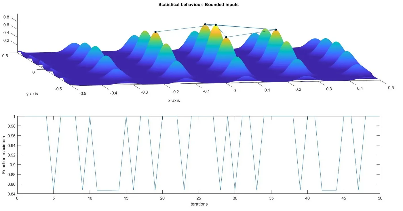
Significant improvements are seen after defining the lower and upper bounds. Once the algorithm is demanded to search only in a specific region, it is able to produce much more accurate results. The output above is not the sought solution by any means, however, the algorithm is now able to evaluate the optimal solution more closely. For instance, the predicted function maximum is now between 0.85 and 1, as opposed to being between 0 and 1 in the first output, which was an unfeasible result.

To optimize further, the initial population size needs to be considered. Because GA starts with random samples, it takes 50 as the number of samples by default, since that is the defined number of iterations. The issue with a smaller sample size is that the algorithm will typically be successful in finding the local maxima(s) rather than the global maxima, which is what happened in Output 2. In order to converge to the optimal solution, which is the global maxima, the initial population size needs to be increased.

Study 3: Statistical behaviour - bounded inputs and increased population size

clear all; close all; clc

x = linspace(-0.5,0.5,200);
y = linspace(-0.5,0.5,200);
num_its = 50;

[xx,yy] = meshgrid(x,y); %creating a 2D array

for i = 1:length(xx) %for every value of x, every value of y will be taken into account
    for j = 1:length(yy)
        input_vector(1) = xx(i,j); %a row vector with 2 columns is created to store the values generated
        input_vector(2) = yy(i,j);      
        f(i,j) = stalagmite(input_vector);
    end
end

%Study 3: increasing population size
options = optimoptions('ga');
options = optimoptions(options,'PopulationSize',200);

tic
for k = 1:num_its
    [coordinates, fval] = ga(@stalagmite,2,[],[],[],[],[-0.2;-0.2],[0.35;0.35],[],[],options);
    xopt(k) = coordinates(1);
    yopt(k) = coordinates(2);
    fopt(k) = -fval;
end

study3_time = toc;

figure(3)
subplot(2,1,1)
hold on
surfc(xx,yy,-f) %multiplying by -1 to plot the actual stalagmite function
shading interp
plot3(xopt,yopt,fopt,'marker','o','markersize',5,'markerfacecolor','k')
title('Statistical behaviour: Bounded inputs with increased population size')
xlabel('x-axis')
ylabel('y-axis')
subplot(2,1,2)
plot(fopt)
xlabel('Iterations')
ylabel('Function maximum')

Referring to the code above, the population size has been increased to 200. It is to be noted that a better defined lower and upper bound would've certainly produce a more optimized result in Study 2, in which case optimization in Study 3 would be easier and perhaps increasing the population size to around a 100 could've been sufficient to obtain the optimal solution. The drawback of a big population size like 200 is that it slows down the algorithm, because a lot more samples need to be processed.

Output 3:

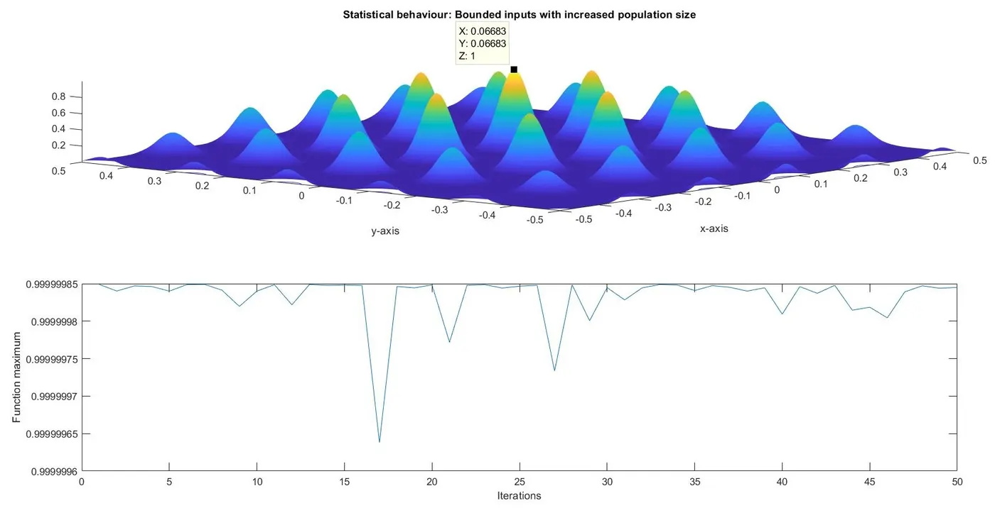
As is evident in Output 3 above, with a higher initial population the algorithm is able to converge to the optimal solution and determine the global maxima (indicated by the black dot in the surface plot). In the graphical plot, it is visible that the algorithm consistently revolves around the global maxima of 1 throughout the 50 iterations.

Conclusion:

Statistical behaviour of the algorithm and the process of optimization to find the global maxima of the stalagmite function was done in three progressive studies as represented above. Through defining lower & upper bounds and increasing initial population size, the optimal solution was found i.e. the coordinates at which the global maximum of the function exists by the end of Study 3.