Curve Fitting and Data Prediction using MATLAB

Aim:

• Write a program to perform curve fitting of linear and cubic polynomials given a large data set.

Objectives:

• Plot linear and cubic fit curves along with the original data points
• Use splitwise method to see comparison of curve fitting with and without the method
• Calculate the error between original data and curve fit

Theory and Governing Equations:

Curve fitting is the procedure of constructing a curve that is in close proximity with the real data. It can also be used to describe how the data changes mathematically and is highly effective in modelling several processes.

There are ways to measure fitness characteristics and goodness of fit of the curve:

• Sum of Squares due to Error (SSE): measure of the discrepancy between the original data and the predicted model.

`SSE = sum_(i=1)^n =`Error`(i)^2`

• Sum of Squares of Regression (SSR): measure of the difference between the value of the predicted model at a given point and the arithmetic mean of the original data set.

`SSR = sum_(i=1)^n [f(x(i)) - Mean]^2`

• R-square: a statistical measurement between 0 and 1 of how close the original data is to the predicted model.

`R^2 = (SSR)/(SSR + SSE)`

• Root Mean Squared Error (RMSE): estimate of the standard deviation of the random component in the data.

`RMSE = sqrt((SSE)/n)` [where n = number of data points]

*The given data set consists of 3200 values of temperature and specific heat, and will be used in this project this point onwards.

Linear curve fit:

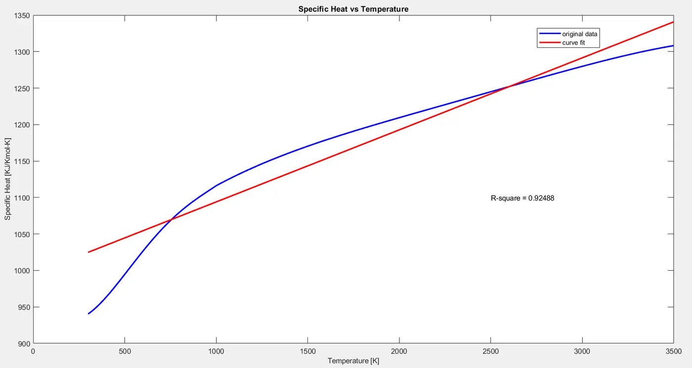
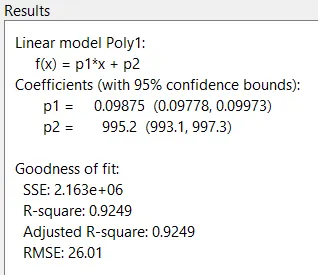
As is also evident from the R square value of 0.92488 (<<0.95), which has been verified with the inbuilt curve fitting tool, a linear model is clearly not a good fit for the given data.

Code for cubic curve fit:

clear all
close all
clc

cp_data = load('data');
temp = cp_data(:,1);
cp = cp_data(:,2);

plot(temp,cp,'linewidth',2,'color','b')
hold on
xlabel('Temperature [K]','fontsize',10)
ylabel('Specific Heat [KJ/Kmol-K]','fontsize',10)
title('Specific Heat vs Temperature [For cubic curve fit *without* splitwise method]','fontsize',10)

%assuming cp = a*T^3 + b*T^2 + cT + d;
[coeff,S,mu] = polyfit(temp,cp,3); %the input array of [coeff,S,mu] helps to avoid an ill-conditioned polynomial through a centering and scaling transformation
predicted_cp = polyval(coeff,temp,S,mu);

%finding the error between data and the curve fit
t = table(temp,cp,predicted_cp,cp - predicted_cp,'VariableNames',{'Temp','Cp','Curve_Fit','Error'});

plot(temp,predicted_cp,'linewidth',2,'color','r')
hold off
legend('original data','curve fit')

%R-square to validate the curve fit
total_cp = 0;
for i = 1:length(cp_data(:,1))
    total_cp = total_cp + cp(i);
end

mean = total_cp/3200;

%to calculate sum of squares of regression (SSR)
SSR_3 = 0;
for j = 1:length(cp_data(:,1))
    SSR_3 = SSR_3 + (predicted_cp(j) - mean)^2;
end

%to calculate sum of squares of errors (SSE)
SSE_3 = 0;
for k = 1:length(cp_data(:,1))
    SSE_3 = SSE_3 + (cp(k)- predicted_cp(k))^2;
end

R_square = (SSR_3/(SSR_3 + SSE_3));
text(2000,1100,['R-Square = ' num2str(R_square)], 'fontsize',10)

It is to be noted that the code for linear and cubic fit is essentially the same, with the difference being the varied degree of the polynomial from 1 to 3 within the polyfit command.

However, for a cubic fit, a couple additional lines of codes needed to be considered. For instance, an input array of [coeff,S,mu] instead of just [coeff] needed to be introduced to use the centering and scaling transformation in order to avoid an ill-conditioned polynomial. Another thing implemented for the cubic fit was the calculation of the error between the original data and the curve fit, to understand whether a cubic fit is a solution that could be considered. This was not done for the linear fit because that represents an unfeasible solution, so calculating the error is unnecessary.

Cubic curve fit:

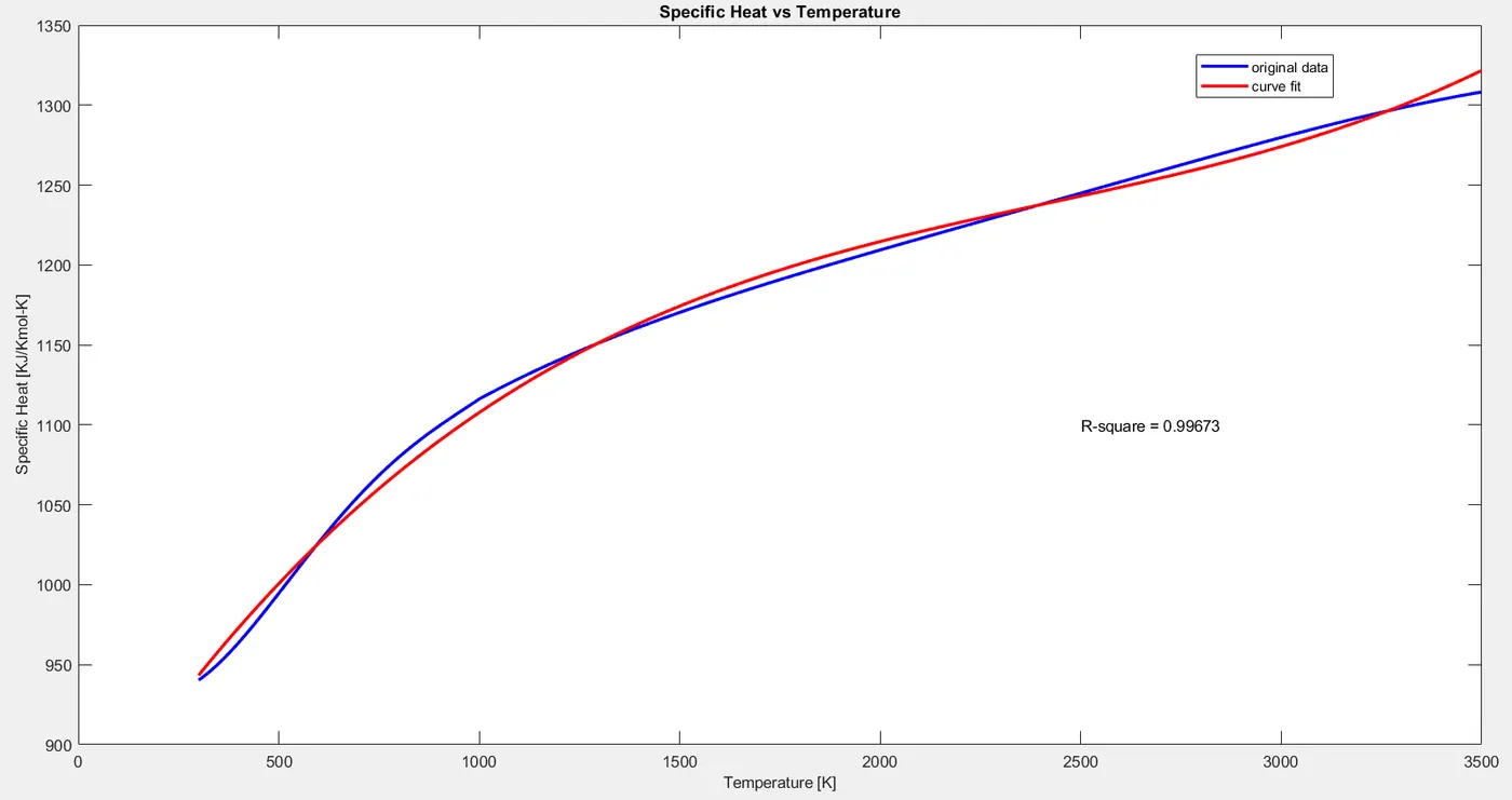
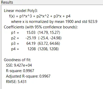
Evidently, this is a much better fit, with the R square value of 0.99673(>>0.95). At this point, it could be realized that a cubic polynomial, with a few tweaks, could potentially be the sought solution for the given data. The curve fit seen above has been generated as a single polynomial function, but there always exists a possibility of inputting multiple polynomials for different ranges, as to customize the curve fit to every part of the data. This is known as the splitwise polynomial method.

Code for cubic curve fit with splitwise method incorporated:

clear all
close all
clc

cp_data = load('data');
temp = cp_data(:,1);
cp = cp_data(:,2);

%splitwise method
temp_1 = cp_data(1:800,1);
cp_1 = cp_data(1:800,2);
temp_2 = cp_data(801:1600,1);
cp_2 = cp_data(801:1600,2);
temp_3 = cp_data(1601:2400,1);
cp_3 = cp_data(1601:2400,2);
temp_4 = cp_data(2401:3200,1);
cp_4 = cp_data(2401:3200,2);

[coeffs_1,S1,mu1] = polyfit(temp_1,cp_1,3);
[coeffs_2,S2,mu2] = polyfit(temp_2,cp_2,3);
[coeffs_3,S3,mu3] = polyfit(temp_3,cp_3,3);
[coeffs_4,S4,mu4] = polyfit(temp_4,cp_4,3);

curve_fit_1 = polyval(coeffs_1,temp_1,S1,mu1);
curve_fit_2 = polyval(coeffs_2,temp_2,S2,mu2);
curve_fit_3 = polyval(coeffs_3,temp_3,S3,mu3);
curve_fit_4 = polyval(coeffs_4,temp_4,S4,mu4);

%finding the error between data and the curve fit
t = table([temp_1 temp_2 temp_3 temp_4],[cp_1 cp_2 cp_3 cp_4],[curve_fit_1 curve_fit_2 curve_fit_3 curve_fit_4],[cp_1 - curve_fit_1 cp_2 - curve_fit_2 cp_3 - curve_fit_3 cp_4 - curve_fit_4],'VariableNames',{'Temp','Cp','Curve_Fit','Error'});
plot(temp,cp,'--','color','b','linew',1.5)
hold on
xlabel('Temperature [K]','fontsize',10)
ylabel('Specific Heat [KJ/Kmol-K]','fontsize',10)
title('Specific Heat vs Temperature [For cubic curve fit *with* splitwise method]','fontsize',10)
plot([temp_1 temp_2 temp_3 temp_4],[curve_fit_1 curve_fit_2 curve_fit_3 curve_fit_4],'r--','linew',1.5)
legend('original data','curve fit')

%R-square to validate the curve fit
total_cp = 0;
for i = 1:800
    total_cp_1 = total_cp + cp_1(i); %summation of cp values for first split
    total_cp_2 = total_cp + cp_2(i);
    total_cp_3 = total_cp + cp_3(i);
    total_cp_4 = total_cp + cp_4(i);
end

mean_1 = total_cp_1/800; %mean of cp values for first split
mean_2 = total_cp_2/800;
mean_3 = total_cp_3/800;
mean_4 = total_cp_4/800;

%to calculate sum of squares of regression (SSR)
SSR = 0;
for j = 1:800
    SSR = SSR + (curve_fit_1(j) - mean_1)^2;
    SSR = SSR + (curve_fit_2(j) - mean_2)^2;
    SSR = SSR + (curve_fit_3(j) - mean_3)^2;
    SSR = SSR + (curve_fit_4(j) - mean_4)^2;
end

%to calculate sum of squares of errors (SSE)
SSE = 0;
for k = 1:800
    SSE = SSE + (cp_1(k) - curve_fit_1(k))^2;
    SSE = SSE + (cp_2(k) - curve_fit_2(k))^2;
    SSE = SSE + (cp_3(k) - curve_fit_3(k))^2;
    SSE = SSE + (cp_4(k) - curve_fit_4(k))^2;
end

R_square = (SSR/(SSR+SSE));
text(2500,1100,['R-Square = ' num2str(R_square)], 'fontsize',10)

Output and comparison:

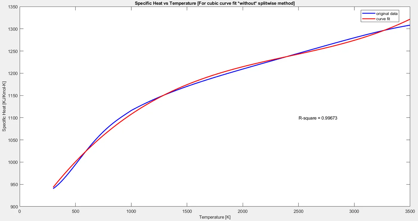
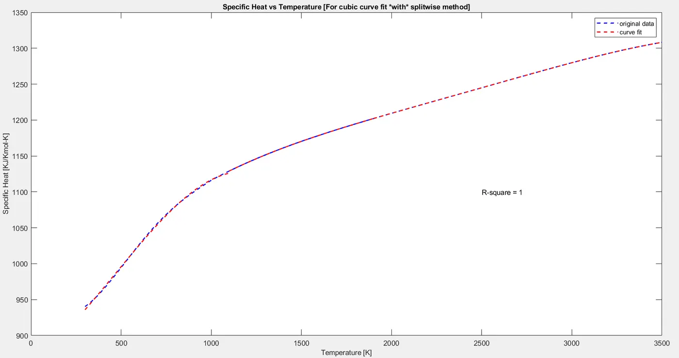
As visible in the comparison above and backed by their respective R-square values, curves of the same polynomial degree can be fitted better with the splitwise method. It is to also be noted that the preciseness of the splitwise method can be further improved through better splitting of the given data. For example, for the curve fit above, the data was split into four equal segments of 800 data points each. However, if closer attention was paid to the inflection points of the original data, and then appropriate segmentation was done accordingly, a better result could be obtained for higher precision.

Without and with the splitwise method, the margin of errors between the data points can also be seen, respectively:

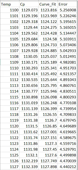
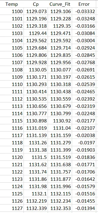
Above is a random selection of data points to demonstrate the comparison. This showcases the effectiveness of the splitwise method in improving the accuracy of the curve fit.

Questions:

• How to make a curve fit perfectly?

A perfect fit implies that there is negligible difference between the original data and the fitted curve. In order to do this, error estimates also need to be considered. Usually, increasing the degree of the polynomial leads to a perfect fit. However, with this method, there is a chance that the curve fit fails beyond the original data set range and cannot act as an effective modelling and prediction technique beyond a given range. This is due to the inbuilt polynomial function, which when exposed to a high degree, tries to exactly fit the original data to satisfy the code's demand, but might diverge, converge or falter if a higher range is inputted. On the other hand, splitwise polynomial method seems to be a more feasible procedure to obtain a perfect fit, as it uses the process of segmentation.

• How to get the best fit?

There are four quantificators which assist in achieving the best fit of a constructed curve:

a) Sum of Squares due to Error (SSE)

b) R-square

c) Adjusted R-square

d) Root Mean Squared Error (RMSE)

*Typically, lower the SSE and RMSE, and higher the R-square, the better the fit will be.

• What could be done to improve the cubic fit?

As has been demonstrated and explained above, splitwise polynomial method is extremely effective in improving the cubic fit.

Conclusion:

Codes have been written to fit a linear and cubic polynomial for the given data set. A linear fit is not the appropriate solution, while the cubic fit is the sought solution when the splitwise polynomial method is considered.