Otto Cycle representation using MATLAB

Introduction

The Otto cycle is an idealized thermodynamic cycle that is commonly found in automobile petrol engines. It involves spark ignition, where constant volume heat addition and heat rejection takes place.

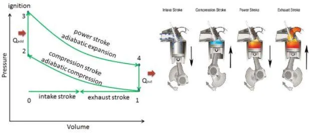
Pressure and volume at each state i, would be pi, vi

Generally, when studies are performed for an Otto cycle, volumes v1 and v2 are calculated simply using the bore and stroke dimensions to find swept and clearence volumes. Since it is a constant volume process, v1 = v4 and v2 = v3. The pressures can be found as well at these locations easily using the ideal gas laws and the formula pv^gamma = constant. Nevertheless, the actual compression and expension processes are hard to physically draw and plot on a graph.

Using MATLAB, it is possible to run a volume trace between each state, to obtain the true plot of the otto cycle. This will be demonstrated in this project by creating and calling a function to capture this volme trace.

Code:

The main code written is provided below, with clear explainations of the processes provided in the code itself:

clear all
close all
clc
%1-2 isentropic compression
%2-3 constant volume heat addition
%3-4 isentropic expansion
%4-1 constant volume heat rejection

%inputs
gamma = 1.4;
t3 = 2300; %kelvin, the highest temperature due to spark ignition)

%variables at state 1- compression begins
p1 = 101325; %Pa
t1 = 500; %K

%geometric parameters of the engine
bore = 0.1;  %meter
stroke = 0.1; %meter
c_rod = 0.15; %meter
cr = 12; %compression ratio

%swept and clearence volumes
v_swept = (pi/4)*bore^2*stroke;
v_clearence = v_swept/(cr-1);

v1 = v_clearence + v_swept;
v2 = v_clearence;

c = p1*(v1^gamma); %constant for isentropic compression

%variables at state 2 (after compression has taken place)
%p1*(v1^gamma) = p2*(v2^gamma)
p2 = p1*(cr^gamma);
%using ideal gas law, (p2*v2)/t2 = (p1*v1)/t1
t2 = (p2*v2*t1)/(p1*v1);
%now we call the volume trace function for compression, varying from 180-0
V_compression = engine_kinematics(bore,stroke,c_rod,cr,180,0);
P_compression= c./V_compression.^gamma; %as pv^gamma is a constant

%variables at state3, (after constant volume heat addition)
v3 = v2; %constant volume heat addition for an otto cycle
%(p3*v3)/t3 = (p2*v2)/t2, ideal gas law
p3 = (p2*t3)/t2;

%variables at state 4 (after isentropic expansion)
v4 = v1;

e = p3*(v3^gamma);
%we need to call the vol trace function for expansion, from 180 to 360 deg
V_expansion = engine_kinematics(bore,stroke,c_rod,cr,0,180);
P_expansion= e./V_expansion.^gamma; %as pv^gamma is a constant

%p3*(v3^gamma) = p4*(v4^gamma)
p4 = p3*(v3/v4)^gamma;


plot([v1, V_compression],[p1, P_compression],[v2, v3],[p2, p3],[V_expansion, v4],[P_expansion, p4],[v4, v1],[p4, p1],'linewidth',3)
title('Otto Cycle')
xlabel('V in m3')
ylabel('P in pa')
text(v1,p1,'1')
text(v2,p2,'2')
text(v3,p3,'3')
text(v4,p4,'4')

Note - A function engine_kinematics is called upon.

Using this function, the crank angle can be varied to suction and compression angles accordingly. This is beneficial to obtain the volume trace and get the curved path of expansion and compression.

If only values v1 v2 v3 v4, p1 p2 p3 p4, are calculated and plotted, the plot would simply comprise of straight lines, which is wrong.

function [V] = engine_kinematics(bore,stroke,c_rod,cr,start_angle,end_angle)

%this is a function that can be called upon for use for a volume trace

a = stroke/2;
R = c_rod/a;

v_swept = (pi/4)*bore^2*stroke;
v_clearence = v_swept/(cr-1);

theta = linspace(start_angle,end_angle,100);
term1 = 0.5*(cr-1);
term2 = R + 1 - cosd(theta);
term3 = (R^2 - sind(theta).^2).^0.5;
V = (1 + term1*(term2-term3)).*v_clearence;
end

Here, V represents the volume trace array and function [V] is solved for by inputing the bore, stroke, connecting rod lengths, along with the compression ratio and start and end angles.

Outputs:

The p-v diagram is obtained:

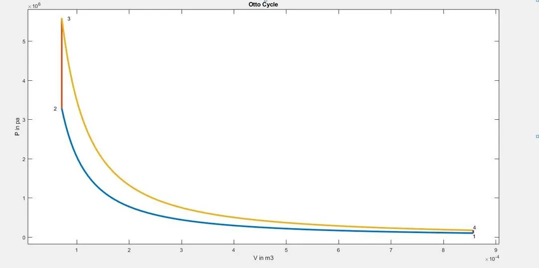
This is a correct representation of the otto cycle. 1-2 represents compression (blue), 2-3 represents heat addition (red), 3-4 represents expansion (yellow), and 4-1 represents heat rejection (purple).

The thermal efficiency was calculated in the command window:

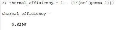
Hence, the thermal efficiency for this otto cycle is around 63%.