Analysis of a Mixing Tee using Ansys Fluent.

Introduction:

The Mixing Tee is a device used to mix the same fluids of two different temperature fluids. Generally in a mixing Tee, There will be Two inlets which may be perpendicular to each other and an outlet. Through the outlet, we will be getting an intermediate temperature compared to temperatures of both the inlets. Standard deviation at the outlet will be a good indicator of the mixing efficiency. The inlet velocity and the length of the tube are the two major factors that are to be considered. We will be doing simulations and study the impact of both these factors in mixing.

Aim:

• To grab knowledge about the usage of appropriate turbulence models.
• To compare the mixing efficiency of two different Mixing Tee geometries (Short one and long one).
• To find out the impact of momentum ratio in the outlet temperature.

Selection of turbulence model.

Here we have to Compare the Standard k-epsilon model and SST k-Omega model. Let's first look into the theory behind these two models. Both the SST k-Omega and Standard k-epsilon models are 2 equation-based models.

In the standard k-ε model, the eddy viscosity is determined from a single turbulence length scale, so the calculated turbulent diffusion is that which occurs only at the specified scale, whereas in reality, all scales of motion will contribute to the turbulent diffusion. The k-e model uses the gradient diffusion hypothesis to relate the Reynolds stresses to the mean velocity gradients and the turbulent viscosity. Performs poorly for complex flows involving severe pressure gradient, separation, strong streamline curvature. The most disturbing weakness is lack of sensitivity to adverse pressure gradients; another shortcoming is numerical stiffness when equations are integrated through the viscous sublayer which is treated with damping functions that have stability issues

This is the default k–ω model. This model allows for a more accurate near-wall treatment with an automatic switch from a wall function to a low-Reynolds number formulation based on grid spacing. Demonstrates superior performance for wall-bounded and low Reynolds number flows. Shows potential for predicting transition. Options account for transitional, free shear, and compressible flows.

K epsilon is best suited for flow away from the wall, say free surface flow region, whereas the k-omega model is best suited for near the wall-flow region, where the adverse pressure gradient is developed. If we are examining k-Omega and k-epsilon equations there is one extra term in the k-Omega equation which is making the difference. in the SST k-Omega model, There is a blending function which will switch between these two models depending on the distance from the wall. So SST k-Omega model will be giving the correct answer.

Comparing the results of both the models.

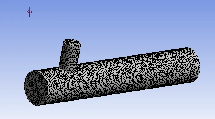
For both cases, short pipe geometry is used with 2mm mesh size. The flow domain is given below.

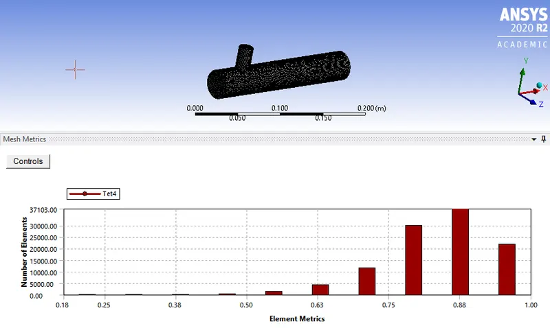
Mesh quality is found to be greater than 18 per cent for all the cases which can be accepted. The Mesh quality report is given below.

The results obtained from both models are given below.

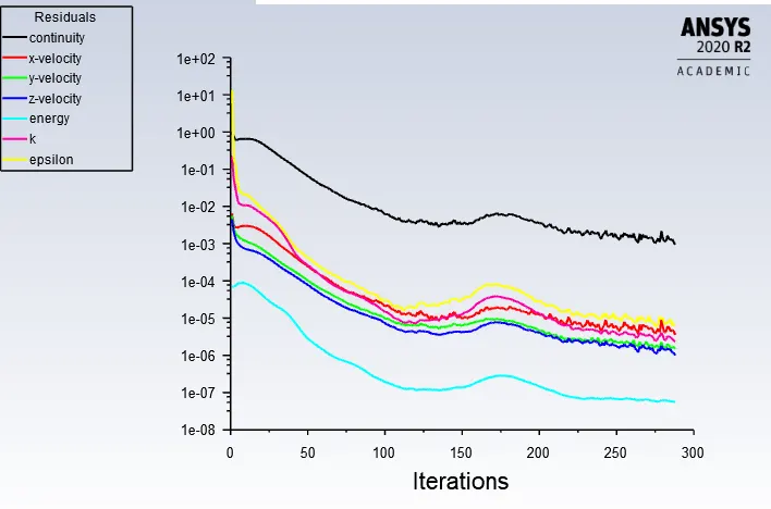
k-epsilon model.

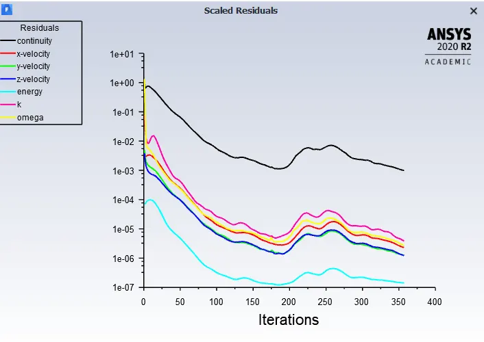
The Convergence plot.

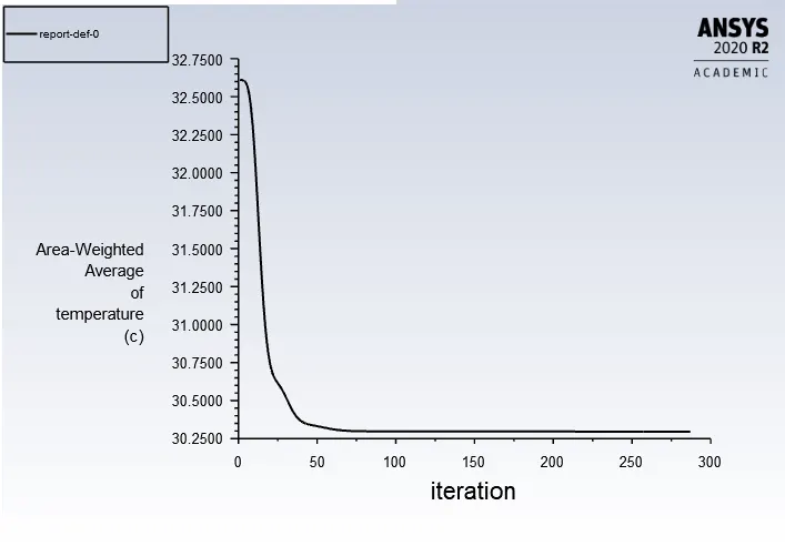
The area-weighted average of temperature at the outlet.

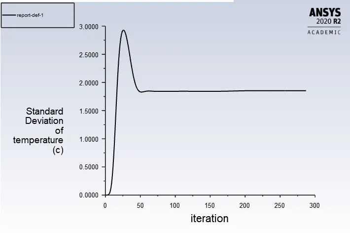
The standard deviation of temperature at the outlet.

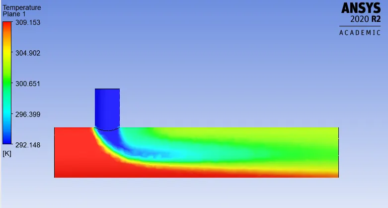
Temperature contour.

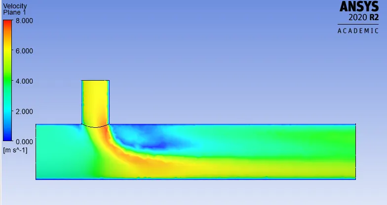
Velocity contour.

k-Omega model.

The Convergence plot.

The area-weighted average of temperature at the outlet.

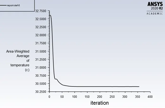
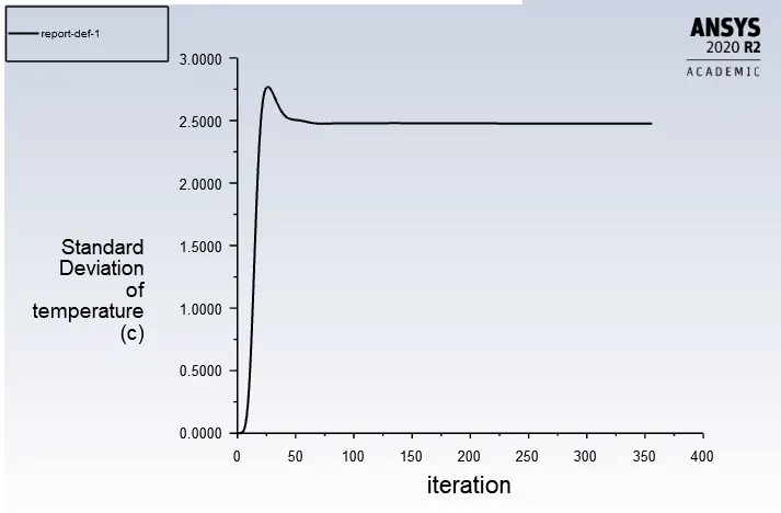
The standard deviation of temperature at the outlet.

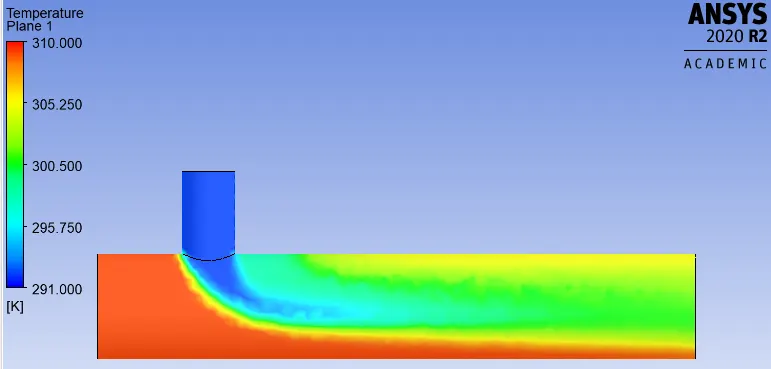
Temperature contour.

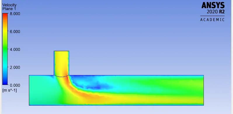
Velocity contour.

Mesh Independence Test

• For the short pipe case Mesh independence test has been done for a momentum ratio of 2.
• Element sizes were 0.3 mm and 0.2 mm respectively.

Comparison of their results is shown below.

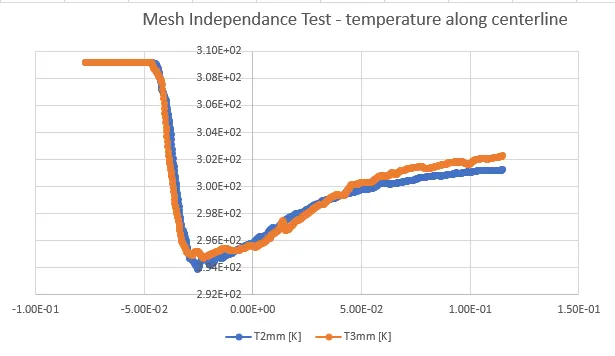
The temperature along the centerline is plotted for both the cases and the curves were almost coinciding. The maximum deviation is found at the outlet and the percentage deviation is just 0.343% which is acceptable. so a 3mm Mesh size is used for further studies. The results for various cases are given below

Short tee - Momentum ratio = 2

Convergence Plot

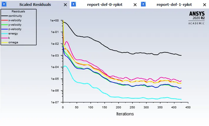
Number of iterations = 430

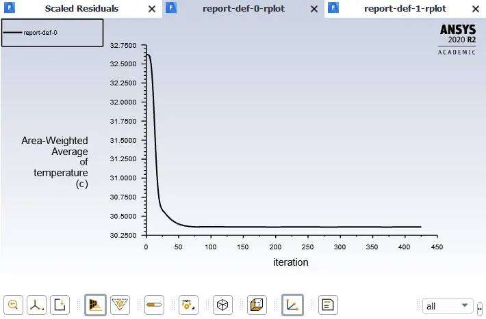
Average outlet temperature = 30.4

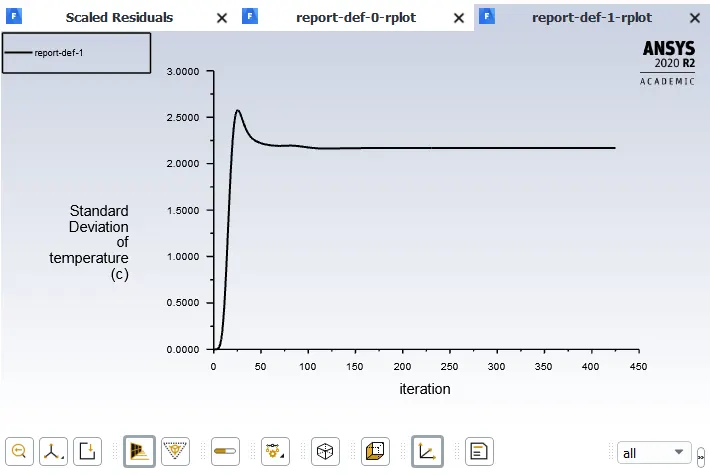
Maximum Standard deviation = 2.625 K.

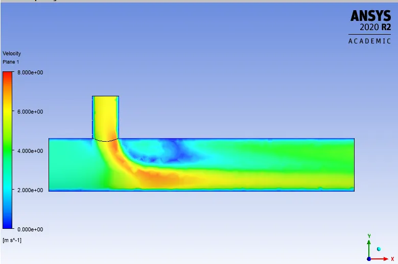
Velocity contour plot along the pipe

Velocity line plot along the pipe

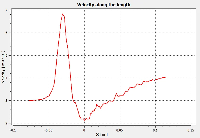
The maximum velocity along the centerline is found to be around 6.75 m/s

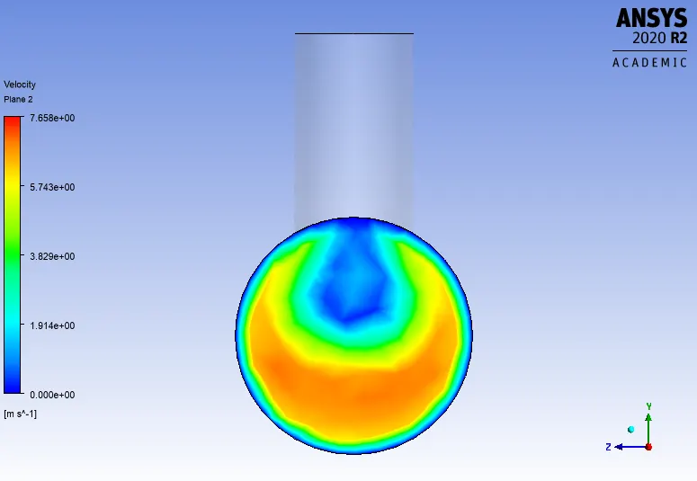
Velocity contour plot across the pipe.

Velocity line plot across the pipe.

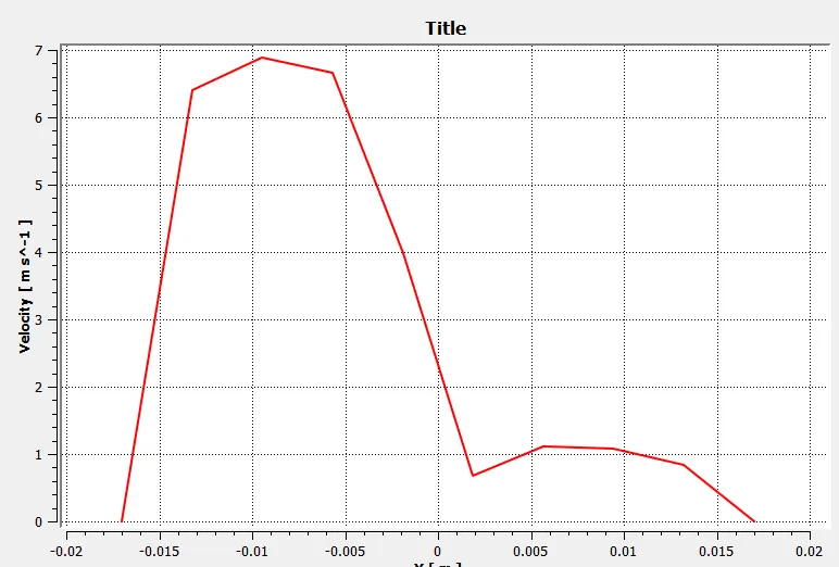
maximum velocity is found around 6.8 m/s in the y-direction on the selected plane.

Temperature contour plot along the pipe

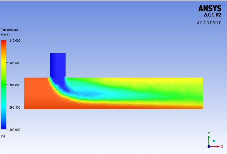
Temperature line plot along the pipe

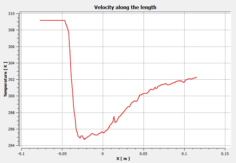
Outlet temperature at the outlet is about 302.5 K

Temperature contour plot across the pipe.

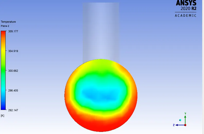
Temperature line plot across the pipe.

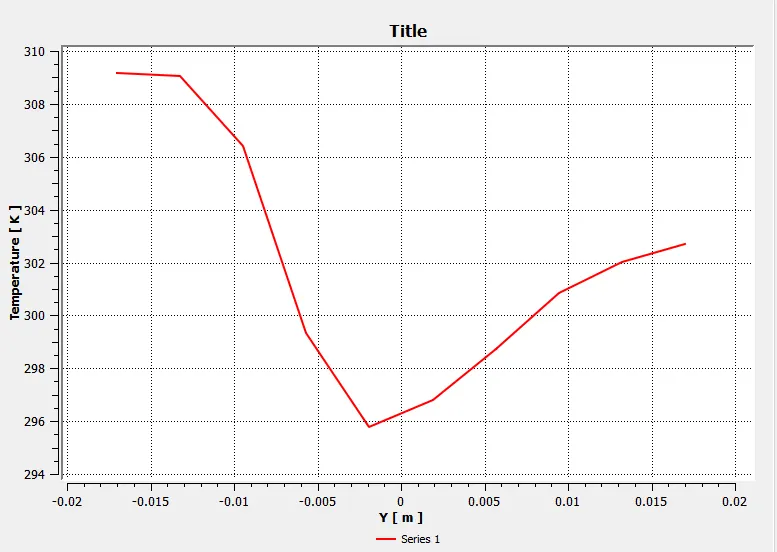
maximum temperature in the selected line is about 309K

Short tee - Momentum ratio = 4

Convergence Plot

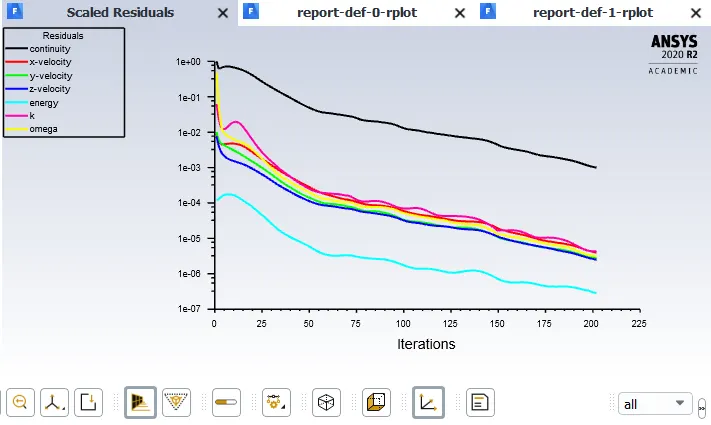
Number of iterations for convergence is around 203

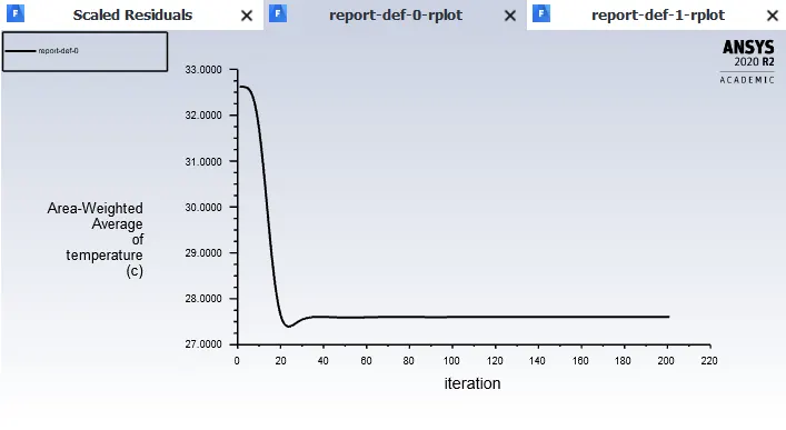
The average outlet temperature is about 27.5-degree celsius.

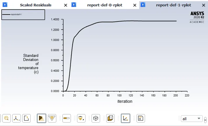
The maximum standard deviation is about 1.3 degrees Celcius.

Velocity contour plot along the pipe

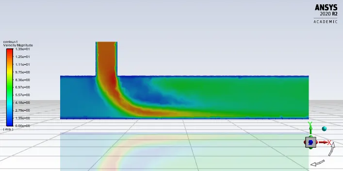
Velocity line plot along the pipe

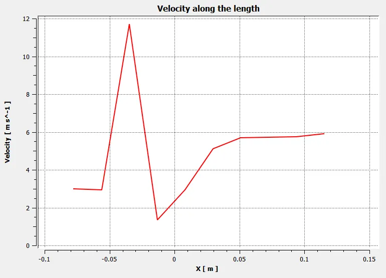
Maximum Velocity a the centre line is about 11.5 m/s and that at the exit is about 6 m/s.

Velocity contour plot across the pipe.

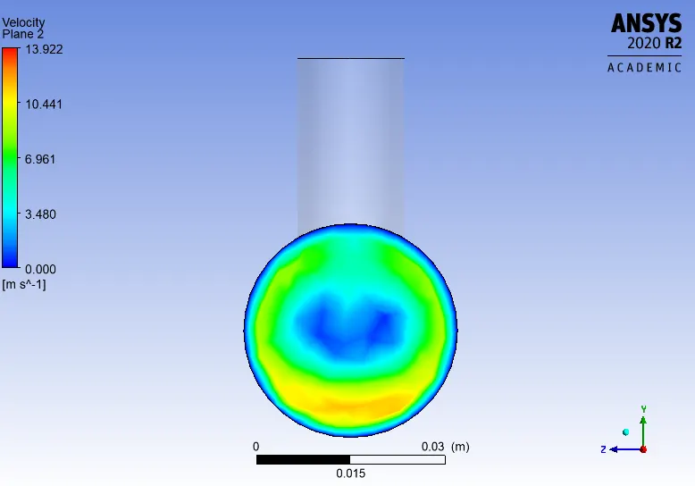
Velocity line plot across the pipe.

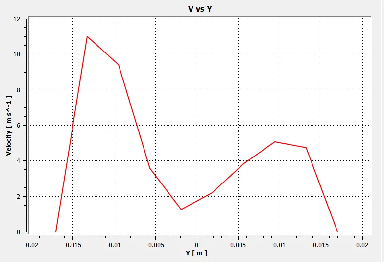
The maximum velocity Along the selected line in the selected plane is around 11 m/s

Temperature contour plot along the pipe

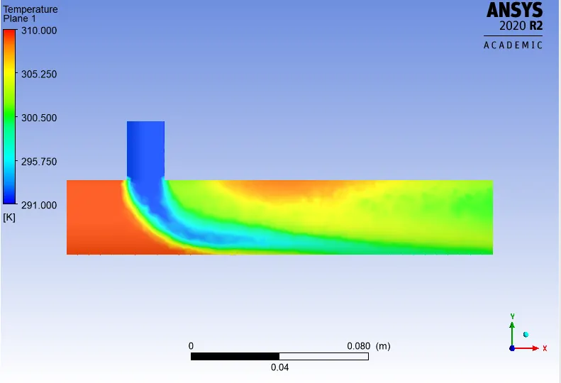
Temperature line plot along the pipe

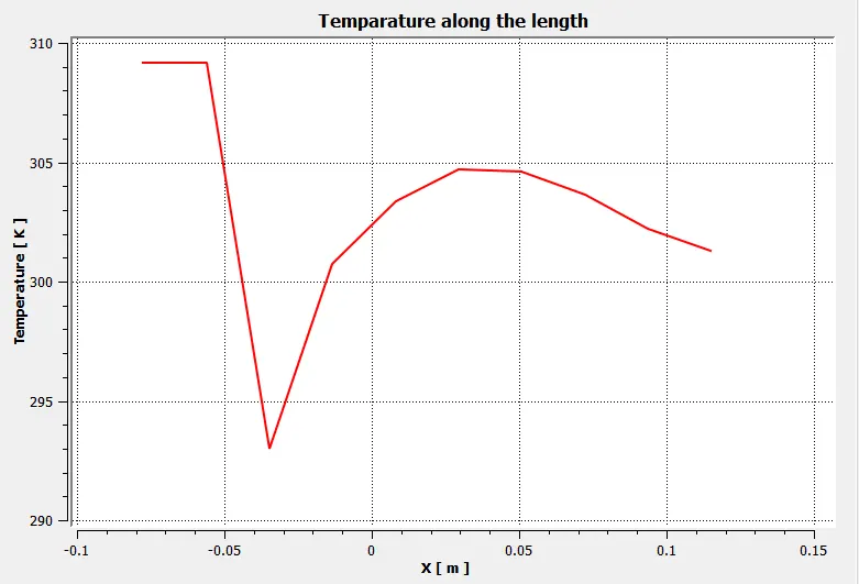
The outlet temperature is around 301.5 K and maximum Temperature is about 309 K.

Temperature contour plot across the pipe.

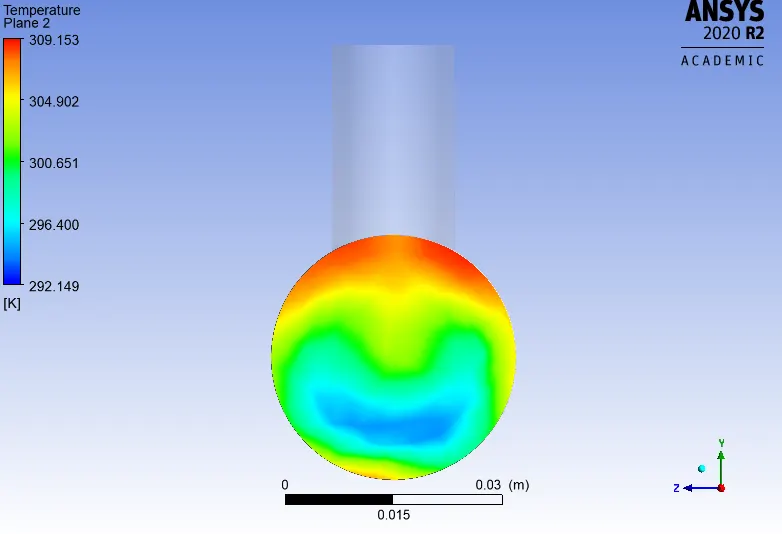
Temperature line plot across the pipe.

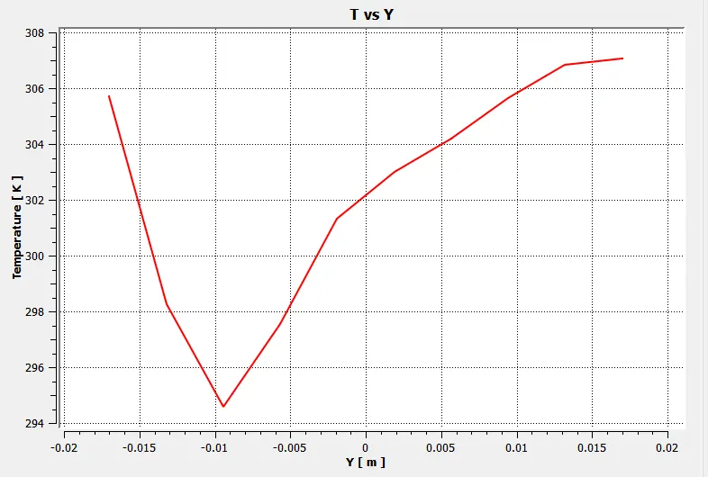
The maximum temperature in the selected line is about 307 K.

Long tee - Momentum ratio = 2

Convergence Plot

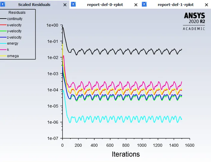
Number of iterations is around 1450

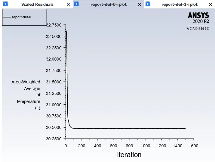
The average outlet temperature is around 30.5 degrees Celcius.

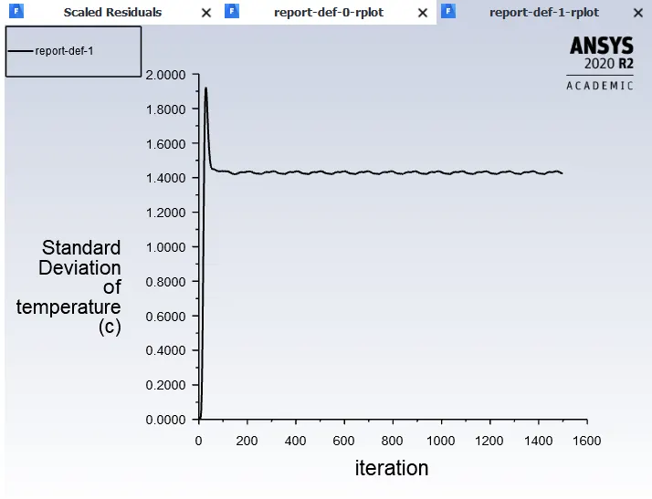
The maximum Standard deviation is around 1.9 degrees Celcius.

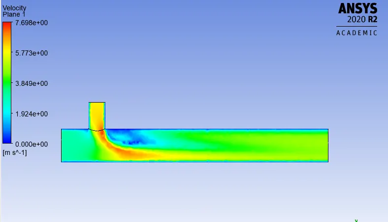
Velocity contour plot along the pipe

Velocity line plot along the pipe

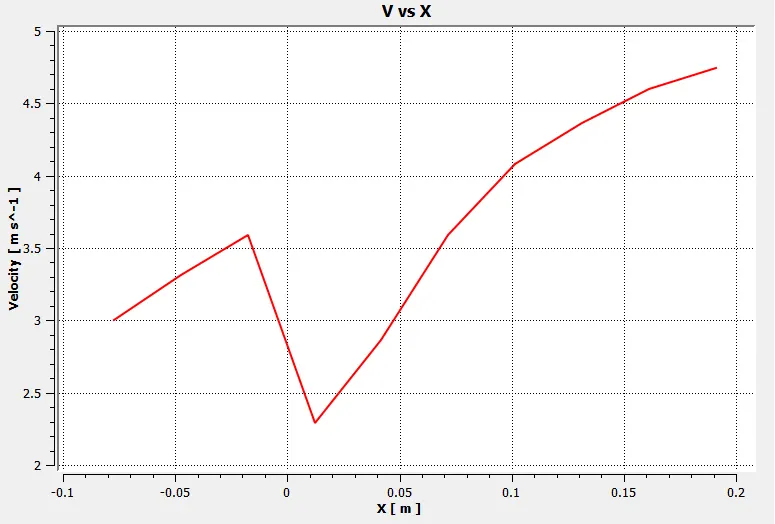
The outlet velocity is found to be 4.56 m/s

Velocity contour plot across the pipe.

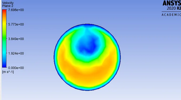
Velocity line plot across the pipe.

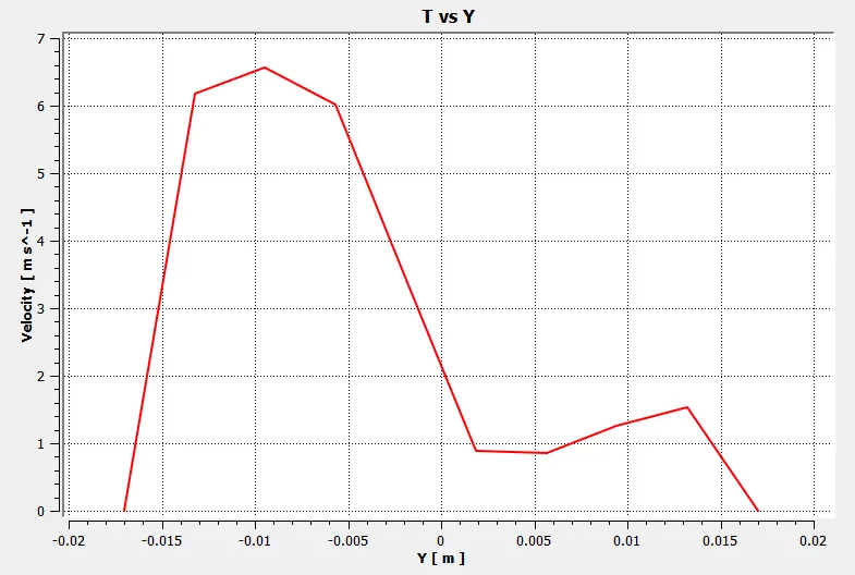
The maximum velocity in the selected line is about 6.5 m/s.

Temperature contour plot along the pipe

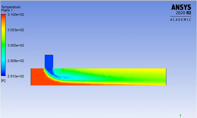
Temperature line plot along the pipe

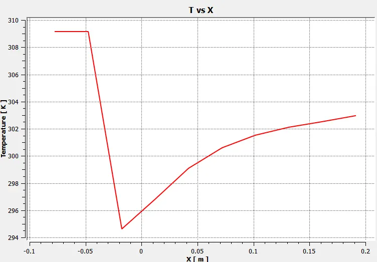
The temperature velocity along the Centerline is about 309K and the outlet temperature is about 303 K.

Temperature contour plot across the pipe.

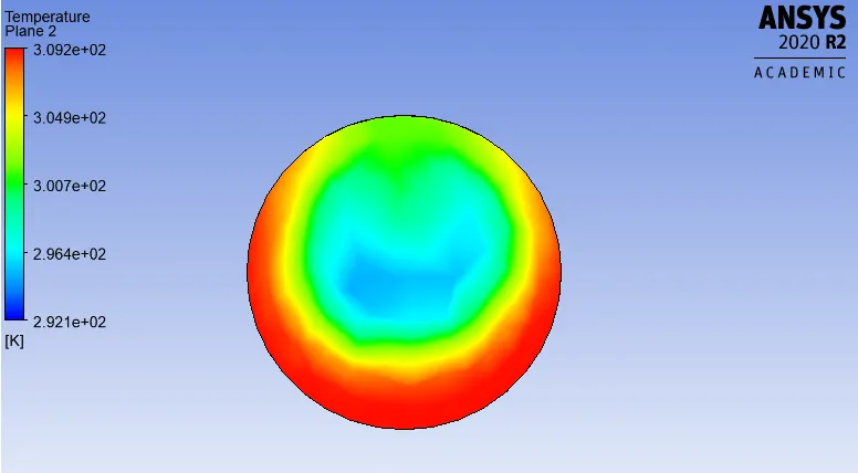
Temperature line plot across the pipe.

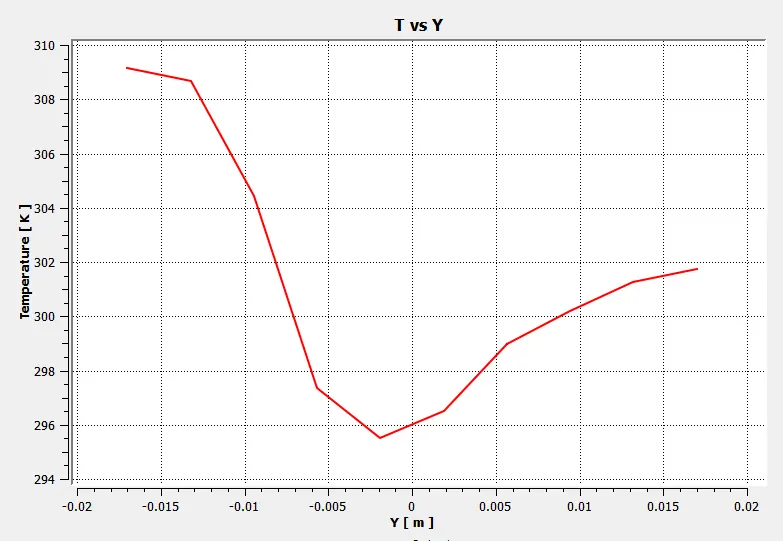
The outlet temperature is around 301.7 K

Long tee - Momentum ratio = 4

Convergence Plot

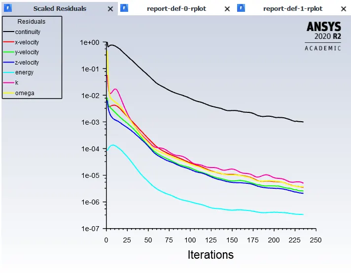
The Number of iteration is about 230

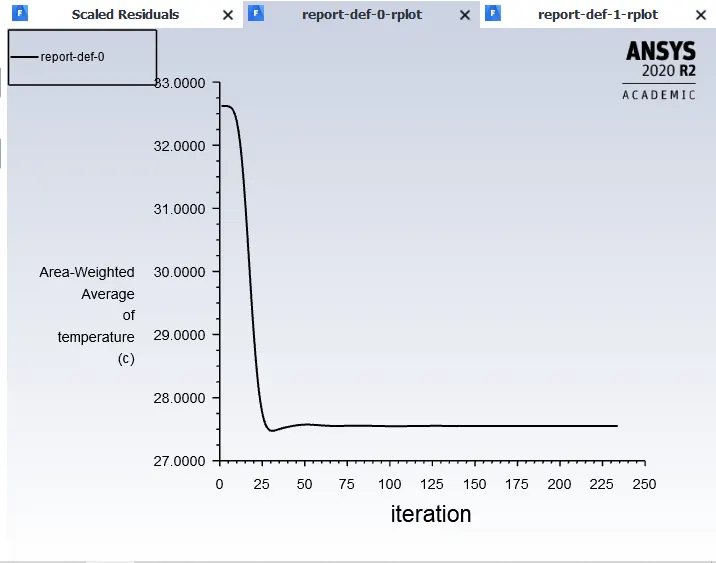
The Average outlet temperature is about 27.56 degrees Celcius.

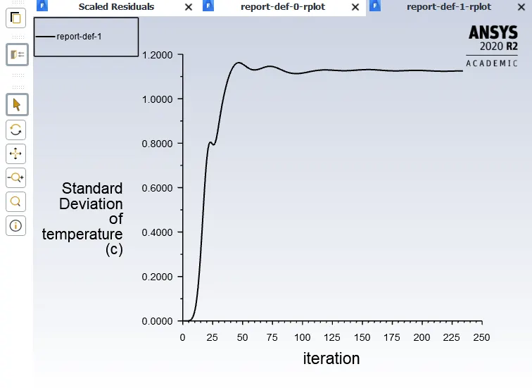
The Maximum Standard deviation is around 1.15 degree Celcius.

Velocity contour plot along the pipe

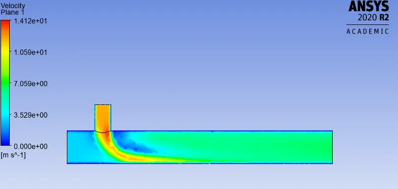
Velocity line plot along the pipe

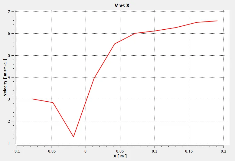
The Outlet velocity is around 6.5 m/s.

Velocity contour plot across the pipe.

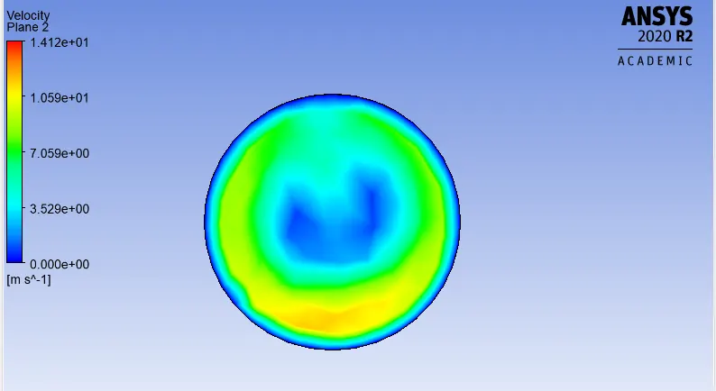
Velocity line plot across the pipe.

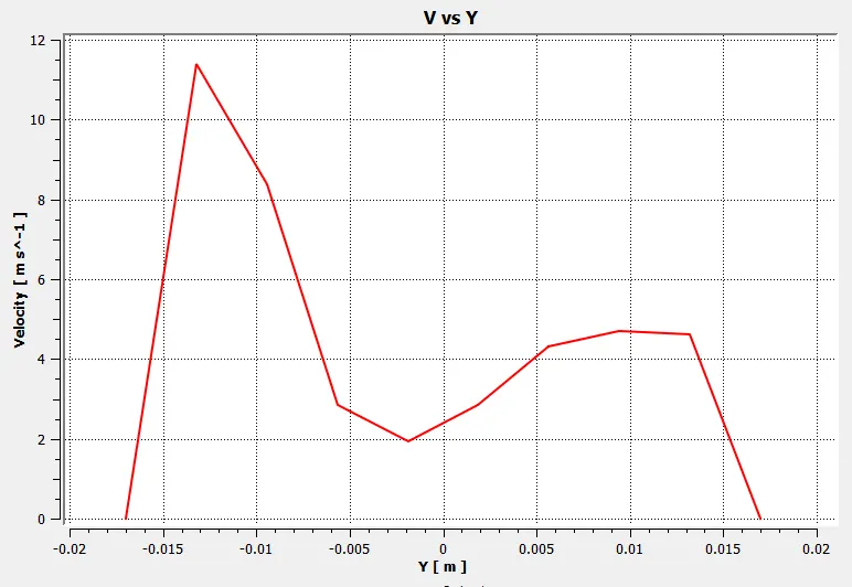
The maximum velocity in the selected line is about 11.25 m/s

Temperature contour plot along the pipe.

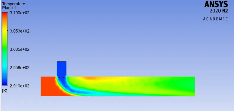
Temperature line plot along the pipe

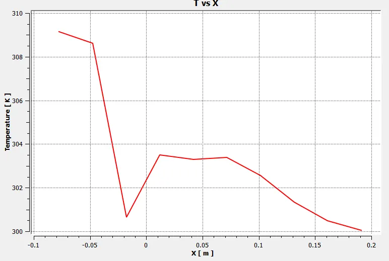
The outlet temperature at the centerline is about 300 K

Temperature contour plot across the pipe.

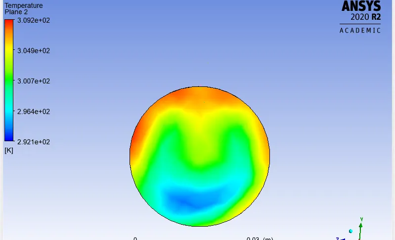
Temperature line plot across the pipe.

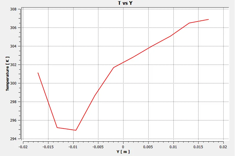
The maximum temperature along the selected line is around 307 K

OBSERVATIONS

	Short Tee Momentum ratio =2	Short Tee Momentum ratio =4	Long Tee Momentum ratio =2	Long Tee Momentum ratio =4
Cell count	39549	39549	56504	56504
Average outlet temperature (degree Celcius)	30.4	27.5	30.5	27.56
Number of iterations for convergence	430	203	241	230
Standard deviation.	2.625	1.3	1.9	1.15

Conclusion

Increase in length causes reduction in standerd deviation which implies better mixing. It's clearly visible in temperature contours.

As the Momentum ratio increases the outlet temperature drops.

For the best results one should use longer tee with higher momentum ratio.