Matlab Programm to solve Air Standard cycle (Otto cycle)

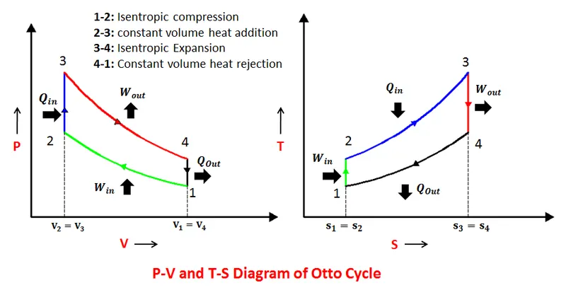
The Otto cycle is executed in a closed system. Neglecting the changes in potential and

kinetic energies, the 1st law of Thermodynamics, on a unit mass base, can be written:

(q_in - q_out)+(W_in - W_out) = du (kJ/kg)

where,

Heat input, q_in = u3 - u2 = Cv(T3-T2)

Heat output, q_out = u4 -u1 = Cv(T4-T1)

Net work done, W_net = q_in - q_out

Thermal efficiency can be calculated as,

η_thermal = w_net / q_in

Thermal efficiency can also be calculated using compression ratio 'r'

η_thermal = 1 - 1/(cr^(γ-1)) ---------- (1)

where, compression ratio cr = V_max/V_min

V_max is maximum value of volume which is, V_max = V1 = V4,

v_min is minimum value of volume which is, V_min = V2 = V3,

and γ (gamma) is adiabatic constant

Typical compression ratios for spark-ignition engines are between 7 and 10. The thermal efficiency increases as compression ratio is increased. However, high compression ratios can lead to auto ignition or engine knock.

Now let's look in the code to calculate all the state variables in otto cycle of a engine.

% Inputs
gamma = 1.4  % adiabatic constant
t3=2300  % in K
% State Variables
p1= 101325 % in pa
t1 =500  % in K

The tempertature at the end of combustion stroke is assumed prior to aid further calculations. This is the highest temperature that can be attained during the cycle. So it is taken as an input.

Geometric parameters of a engine are always fixed for a engine.

so,

% Engine Geometric Parameters
bore= 0.1; % Bore diameter in m
stroke = 0.1; % Stroke length in m
con_rod = 0.15; % connecting rod length in m
cr = 9;

Lets calculate all other initial parameters

% Calculating the swept volume and clerance volume
V_swept = (pi/4)*bore^2*stroke;  % in m^3
V_clerance = V_swept/(cr-1);
V1 = V_swept + V_clerance
V2 = V_clerance

here on variables at the end of every process is calculated in chronology of the cycle,

%State variables at state point 2
%p2v2^gamma = p1v1^gamma -----Adiabatic process
% p2=p1*(V1/V2)^gamma=p1*cr^gamma
 p2 = p1*cr^gamma;
 
%p2V2/t2= p1V1/t1 | t2 = p2*V2*t1/(p1*V1) ----- Ideal gas equation
t2 = (p2*V2*t1)/(p1*V1);

The volume after adiabatic compression is calculated using a seperate function which is defined separately as template named Engine_kinematics

This function will be used calculate volume at compression and expansion. With the help of this function we can plot the volume trace during compression and expansion stroke.

There is a complex formula derived from geometry relations to know the volume at a instant during combustion or exhaust stroke.

which is,

Here,

rc is the compression ratio

R is ratio of connecting rod length and crank pin radius

theta is the crank angle, taken as an array of elements from start of crank and end of crank during process

The code for the same can be written as,

function [V] = Engine_kinematics(bore, stroke, con_rod, cr, start_crank, end_crank)


a = stroke/2; % Crank pin radius
R = con_rod/a; % ratio of connecting rod lengrth and Crank pin radius

% Swept volume and clearance volume 
v_s = pi/4*bore^2*stroke;
v_c = v_s/(cr-1);

% Creating a array of theta to read the position of crank in terms of crank angle.
theta = linspace(start_crank,end_crank,100);

% Calucalting volume at corresponding position of crank
term1 = 0.5*(cr-1);
term2 = R +1 - cosd(theta);
term3 = (R^2 - sind(theta).^2).^0.5;
V = (1+term1*(term2 - term3)).*v_c;

end

During compression stroke crank angle changes from 180 to 0 because piston moves from bottom dead centre to top dead centre.

pressure and volume during compression stroke can be calculated as,

V_compression = Engine_kinematics(bore, stroke, con_rod, cr, 180,0);

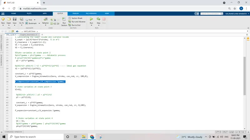
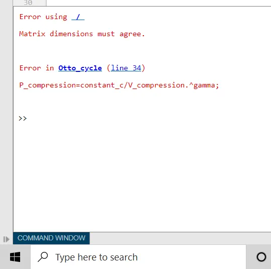
P_compression=constant_c./V_compression.^gamma;

Now heat is added at constant pressure and all the state variables at point 3 can be calculated as,

% state variables at state point 3
V3=V2;

 %p2V2/t2= p3V3/t3 | p3 = p2*t3/t2
 p3 = p2*t3/t2;
 
 constant_c = p3*V3^gamma;

During expansion stroke crank angle changes from 0 to 180 because piston moves from top dead centre to bottom dead centre.

and Pressure and volume changes during expansion stroke can be obtained by the predetermined function Engine Kinematics as below

V_expansion = Engine_kinematics(bore, stroke, con_rod, cr, 0,180);

P_expansion=constant_c./V_expansion.^gamma;

now state variables at the end of expansion stroke can be calculated as

 % State variables at state point 4
 V4 = V1;
 %p3V3^gamma = p4V4^gamma | p4=p3*(V3/V4)^gamma
 p4=p3*(V3/V4)^gamma;

Since we have got all the state variables so lets calculate Thermal efficiency of the cycle

 % calculating thermal efficiency of the cycle
 Thermal_efficiency = (1-cr^(1-gamma))*100;
 fprintf('Thermal efficiency of the cycle in percentage = %d n',Thermal_efficiency);

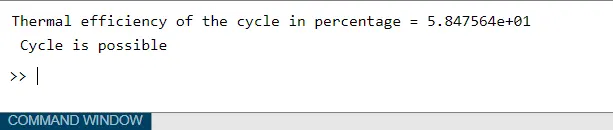
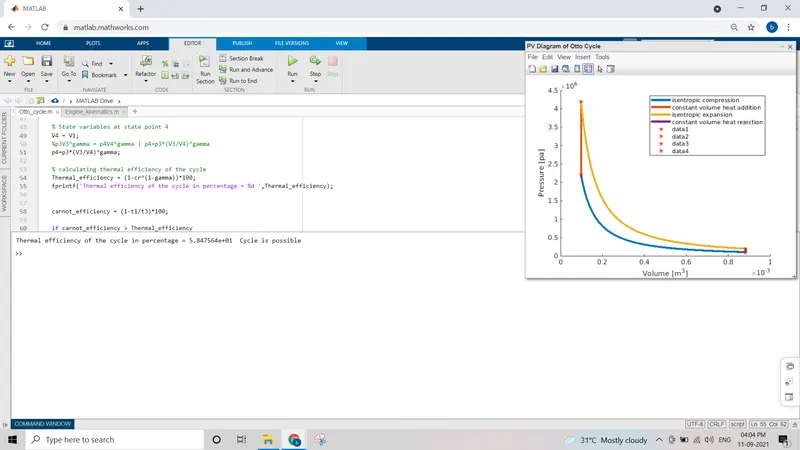
we get, Thermal efficiency = 58.48

This cycle can be cross checked whether it is possible or not by calculating carnot efficiency. Because carnot efficiency give us maximum possible efficiency in a cycle.

 carnot_efficiency = (1-t1/t3)*100;
 
 if carnot_efficiency > Thermal_efficiency
     
     fprintf(' Cycle is possible')
 else
     fprintf('Cycle is impossible')
 end

Now, To plot the PV diagram of the cycle code can be written as,

figure('NumberTitle','off','Name','PV Diagram of Otto Cycle')
 hold on
 plot(V_compression, P_compression,"LineWidth",3)
 plot([V2 V3],[p2 p3],"LineWidth",3)
 plot(V_expansion, P_expansion,"LineWidth",3)
 plot([V1 V4],[p1 p4],"LineWidth",3)
 legend('isentropic compression','constant volume heat addition','isentropic expansion','constant volume heat rejection')
 plot(V1,p1,'*','color','r')
 plot(V2,p2,'*','color','r')
 plot(V3,p3,'*','color','r')
 plot(V4,p4,'*','color','r')
 xlabel('Volume [m^3]')
 ylabel('Pressure [pa]')

Output :

The output we get is

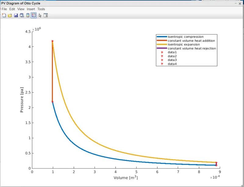
the plot we get is,

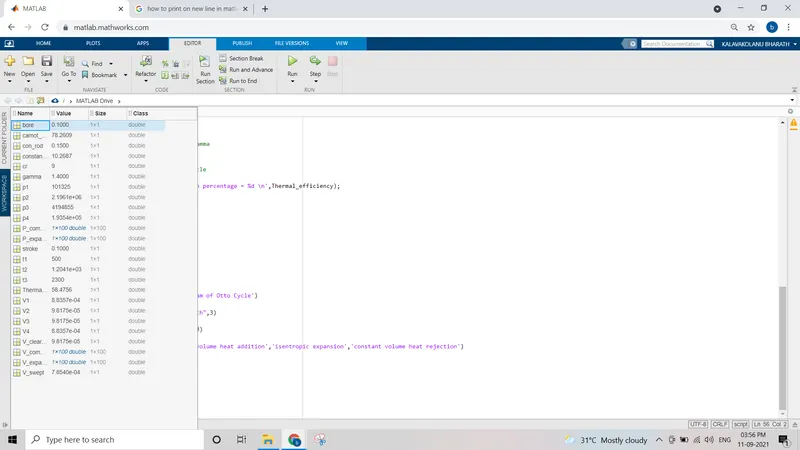
Workspace :

Errors made while programing :

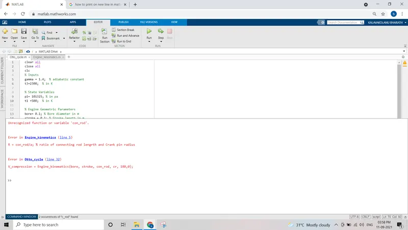
1. There was a typo in Engine_Kinenatics function.

Connecting rod length was named as con_rod in main program but it was uded as c_rod in function code. This was corrected as per main program

2. Missed to use dot operator.

3. Missed to use n to create a new line in output

Conclussion:

1. Thermal efficiency of the cycle is 58.47%

2. PV diagram of the cycle is as shown above.