MATLAB program for Curve Fitting to plot Linear and Cubic polynomials.
AIM:-
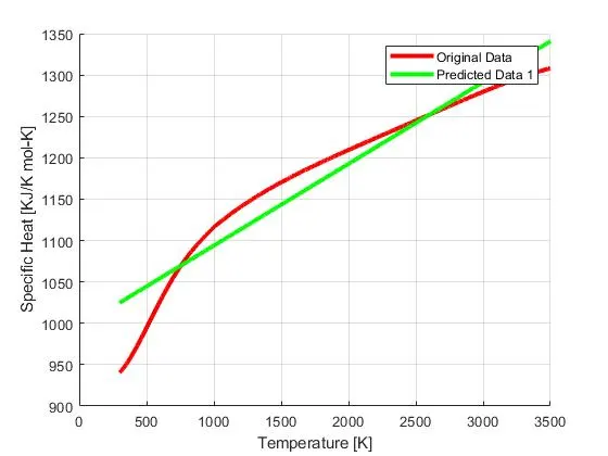
1)Write code to fit a linear and cubic polynomial for the Cp data.
2) Plot the linear and cubic fit curves along with the raw data points. Title and axes labels are a must, legends could be shown if necessary.
3)Write a code to show splitwise method.
THEORY:-
1)Curve fitting:-
Curve fitting is the process of constructing a curve, or mathematical function, that has the best fit to a series of data points, possibly subject to constraints. Curve fitting can involve either interpolation, where an exact fit to the data is required, or smoothing, in which a "smooth" function is constructed that approximately fits the data.
 . A cubic polynomial is a polynomial of degree 3.
%Curve Fitting
clear all
close all
clc
%Input Parameters
data_set=load('data');
temperature=data_set(:,1);
cp=data_set(:,2);
%For Linear polynomial | f=a*x+b
coeffLinear=polyfit(temperature,cp,1);
predicted_data1=polyval(coeffLinear,temperature);
%Comparison Plot
figure(1)
hold on
grid on
plot(temperature,cp,'linewidth',3,'color','r');
plot(temperature,predicted_data1,'linewidth',3,'color','g');
xlabel('Temperature [K]');
ylabel('Specific Heat [KJ/K mol-K]');
legend('Original Data','Predicted Data 1');
%For Cubic polynomial | f=a*x^3+b*x^2+c*x+d
coeffCubic=polyfit(temperature,cp,3);
predicted_data2=polyval(coeffCubic,temperature);
%Comparison Plot
figure(2)
hold on
grid on
plot(temperature,cp,'linewidth',3,'color','r');
plot(temperature,predicted_data2,'linewidth',3,'color','m');
xlabel('Temperature [K]');
ylabel('Specific Heat [KJ/K mol-K]');
legend('Original Data','Predicted Data 2');Explanation:-
1) To proceed with the program, data has to loaded. This is achieved using the load fucntion. Make sure that the data file must be present in the same file registry as the program.
2)Once the different variables are assigned, we use polyfit fucntion to calculate the equation coefficients.
3)Using the coefficients and with the aid of polyval fucntion we calculate new data set, the data that we have predicted.
4)Repetition of the same process to calculate the coefficients and new values for Linear and Cubic polynomials for the curve fit.
5) Plot command is used to generate a graph to assess the data sets and carry out the final conclusion from the data.
6)Legends, axis labels and title is given using the former commands to specifiy and organise the data in the graph
OUTPUT:-
Two plots are generated to aid in visualizing the result.
For linear Polynomial:-
For Cubic Polynomial:-
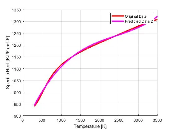
Warning: Polynomial is badly conditioned. Add points with distinct X values, reduce the degree of the polynomial, or try
centering and scaling as described in HELP POLYFIT.
> In polyfit (line 79)
  In curvefit (line 27)
Now, in the cubic plot,the command window shows an error stating that the polynomail is badly conditioned.
"Badly conditioned" means that the solution of the system of linear equations critically depends on rounding errors due to the limited precision.
To get around this error, we use the splitwise method to solve in cubic polynomial.
STEPWISE METHOD:-
This method requires the data to be broken into several ranges. Each range is assigned a new variable and finally all the variables are clubbed togather to generate the final output. This helps to achieve a good curve fit and reduce the error in the function.
Scaling:-
To reduce the "Badly conditioned" error, we can also do scaling. Scaling means to transform the polynomial such that the X-values have a mean of 0 and a standard deviation (or range) of 1.
CODE:-
%Split Wise Method for Curve Fitting
%Input Data
Reading=load('data');
temperature=Reading(:,1);
cp=Reading(:,2);

%Splitwise Method
T1=Reading(1:200,1);
cp1=Reading(1:200,2);
coeff_1=polyfit(T1,cp1,3);
predicted_dat1=polyval(coeff_1,T1);

T2=Reading(201:400,1);
cp2=Reading(201:400,2);
coeff_2=polyfit(T2,cp2,3);
predicted_dat2=polyval(coeff_2,T2);

T3=Reading(401:600,1);
cp3=Reading(401:600,2);
coeff_3=polyfit(T3,cp3,3);
predicted_dat3=polyval(coeff_3,T3);

T4=Reading(601:800,1);
cp4=Reading(601:800,2);
coeff_4=polyfit(T4,cp4,3);
predicted_dat4=polyval(coeff_4,T4);

T5=Reading(801:1000,1);
cp5=Reading(801:1000,2);
coeff_5=polyfit(T5,cp5,3);
predicted_dat5=polyval(coeff_5,T5);

T6=Reading(1001:1200,1);
cp6=Reading(1001:1200,2);
coeff_6=polyfit(T6,cp6,3);
predicted_dat6=polyval(coeff_6,T6);

T7=Reading(1201:1400,1);
cp7=Reading(1201:1400,2);
coeff_7=polyfit(T7,cp7,3);
predicted_dat7=polyval(coeff_7,T7);

T8=Reading(1401:1600,1);
cp8=Reading(1401:1600,2);
coeff_8=polyfit(T8,cp8,3);
predicted_dat8=polyval(coeff_8,T8);

T9=Reading(1601:1800,1);
cp9=Reading(1601:1800,2);
coeff_9=polyfit(T9,cp9,3);
predicted_dat9=polyval(coeff_9,T9);

T10=Reading(1801:2000,1);
cp10=Reading(1801:2000,2);
coeff_10=polyfit(T10,cp10,3);
predicted_dat10=polyval(coeff_10,T10);

T11=Reading(2001:2200,1);
cp11=Reading(2001:2200,2);
coeff_11=polyfit(T11,cp11,3);
predicted_dat11=polyval(coeff_11,T11);

T12=Reading(2201:2400,1);
cp12=Reading(2201:2400,2);
coeff_12=polyfit(T12,cp12,3);
predicted_dat12=polyval(coeff_12,T12);

T13=Reading(2401:2600,1);
cp13=Reading(2401:2600,2);
coeff_13=polyfit(T13,cp13,3);
predicted_dat13=polyval(coeff_13,T13);

T14=Reading(2601:2800,1);
cp14=Reading(2601:2800,2);
coeff_14=polyfit(T14,cp14,3);
predicted_dat14=polyval(coeff_14,T14);

T15=Reading(2801:3000,1);
cp15=Reading(2801:3000,2);
coeff_15=polyfit(T15,cp15,3);
predicted_dat15=polyval(coeff_15,T15);

T16=Reading(3001:3200,1);
cp16=Reading(3001:3200,2);
coeff_16=polyfit(T16,cp16,3);
predicted_dat16=polyval(coeff_16,T16);

%Plotting

%Original Input Data
hold on
plot(temperature,cp,'linewidth',5,'color','y');

%Predicted Data
predicted_dat=[predicted_dat1;predicted_dat2;predicted_dat3;predicted_dat4;predicted_dat5;predicted_dat6;predicted_dat7;predicted_dat8;predicted_dat9;predicted_dat10;predicted_dat11;predicted_dat12;predicted_dat13;predicted_dat14;predicted_dat15;predicted_dat16];
plot(temperature,predicted_dat,'linewidth',3,'color','c');

xlabel('Temperature [K]');
ylabel('Specific Heat [KJ/K mol-K]');
legend('Original Data','Splitwise Data');
title('Temperature vs Specific Heat');
grid on
Explanation:-
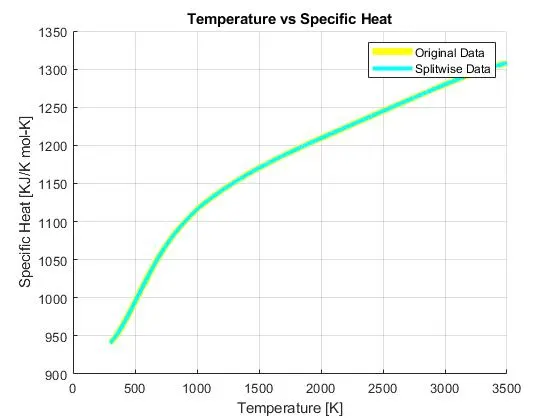
In this code, the range is split in 16 parts to reduce the error. Each new range is assigned a new variable and finally all the new variables are clubbed togather to generate the result.
A plot is generated to and shows the relationship between the original data set and the predicted data set.
OUTPUT:-
Parameters used to measure the fitness characteristics of the curves:-
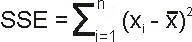
1)The sum of squares due to error(SSE):-
This statistic measures the total deviation of the response values from the fit to the response values. It is also called the summed square of residuals and is usually labeled as SSE. A value closer to 0 indicates a better fit.
The formula for SSE is:
Here,
(X(i)-X(bar))^2 is the error at point i.
2) R sqaure:-
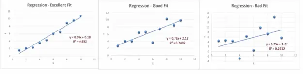
This statistic measures how successful the fit is in explaining the variation of the data. Put another way, R-square is the square of the correlation between the response values and the predicted response values. It is also called the square of the multiple correlation coefficient and the coefficient of multiple determination.
R-square can take on any value between 0 and 1, with a value closer to 1 indicating a better fit. For example, an R2 value of 0.8234 means that the fit explains 82.34% of the total variation in the data about the average.
R-square is defined as the ratio of the sum of squares of the regression (SSR) and the total sum of squares (SST).
3) Adjusted R- square:-
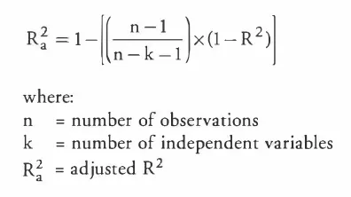
The adjusted R-squared is a modified version of R-squared that has been adjusted for the number of predictors in the model. The adjusted R-squared increases only if the new term improves the model more than would be expected by chance. It decreases when a predictor improves the model by less than expected by chance. The adjusted R-squared can be negative, but it’s usually not. It is always lower than the R-squared.
Case 1,
As k value increases, the value of R-square wil change very less,if the added variable is insignificant. Hence, adjusted R-squared value will decrease.
Case2,
As k value increases, the value of R-square wil increase greatly,if the added variable is significant. Hence, adjusted R-squared value will increase.
4) Root Mean Square Error:-
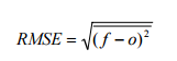
Root Mean Square Error (RMSE) is the standard deviation of the residuals(prediction errors). Residuals are a measure of how far from the regression line data points are; RMSE is a measure of how spread out these residuals are. In other words, it tells you how concentrated the data is around the line of best fit. Root mean square error is commonly used in climatology, forecasting, and regression analysis to verify experimental results.
Where:
- f = forecasts (expected values or unknown results),
- o = observed values (known results).
The bar above the squared differences is the mean (similar to x̄). The same formula can be written with the following, slightly different, notation (Barnston, 1992):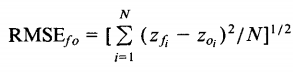
Where:
- Σ = summation(“add up”)
- (zfi – Zoi)2 = differences, squared
- N = sample size.
CONCLUSION:-
1) To fit a curve perfectly, make sure to select the correct value of the order of the polynomial. Measure the error estimates from the above mentioned parameters. Reduce the error, that is the error should be zero and this distance of the points from the curve should be zero, meaning that the data point must lay on the line.
2) To get a best fit, use the curve fitting tool box and select the X Data and Y Data. And generate the code. Compare the values with the help of the fitness parameters and select the best fit. Best fit means to select the most appropriate set of data points, that give the minimum error estimate. Perfect fit is defined as the fit having no errors, meaning all the data points lay on the curve.
3) To improve the cubic, use the splitwise method to split the data in selected no. of ranges or "part" and store them in some variable. For the result, plot all the variables togather.
REFERENCES:-
[4] https://skill-lync.com/projects/Curve-Fitting-and-criterion-to-choose-best-fit-41860
[5] https://skill-lync.freshdesk.com/support/solutions/articles/43000584172