MATLAB program to plot the Otto Cycle and calculate the thermal efficiency.
AIM:- Write code that can solve an otto cycle and make plots for it.
THEORY:-
1) Otto cycle:-
An Otto cycle is an idealized thermodynamic cycle that describes the functioning of a typical spark ignition piston engine. It is the thermodynamic cycle most commonly found in automobile engines.
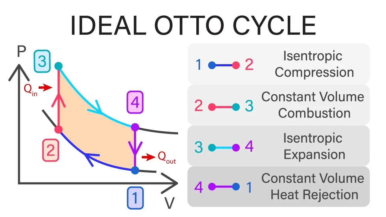
here,
a)Process 1-2 is an adiabatic (isentropic) compression of the charge as the piston moves from bottom dead center (BDC) to top dead center (TDC).
b) Process 2–3 is a constant-volume heat transfer to the working gas from an external source while the piston is at top dead center. This process is intended to represent the ignition of the fuel-air mixture and the subsequent rapid burning.
c) Process 3–4 is an adiabatic (isentropic) expansion (power stroke).
d) Process 4–1 completes the cycle by a constant-volume process in which heat is rejected from the air while the piston is at bottom dead center.
2) BDC:- The point at which the piston of an engine is nearest to the axis of the crankshaft. On a vertical engine, this is the lowest point that the piston reaches.
3) TDC:- The position of an engine's piston when it is at the very top of its stroke.The piston is said to be at top dead center when it has moved to a position where the cylinder volume is a minimum.
4) Swept volume:-The volume through which a piston or plunger moves as it makes a stroke.
5)Clearance Volume:-It is the volume between the cylinder head and the piston top when the piston is at top dead center (TDC). It can also be defined as the volume of cylinder that is not swept by the piston.
6) Compression ratio:- The ratio of the maximum to minimum volume in the cylinder of an internal combustion engine.
7)Adiabatic Index:- It is the ratio of the heat capacity at constant pressure (CP) to heat capacity at constant volume (CV).It is denoted by "gamma".
8) Thermal efficiency:-The efficiency of a heat engine measured by the ratio of the work done by it to the heat supplied to it.
CODE INPUT:-
a)
clear all
close all
clc
 %input data
 gamma=1.4
 t3=2300
 %state variables
 p1=101325
 t1=500
 %engine geometric parameters
 bore=0.1;
 stroke=0.1;
 con_rod=0.15;
 cr=12;
 %Calculating the swept volumeand clearance volume
 v_swept=(pi/4)*bore^2*stroke;
 v_clearance=v_swept/(cr-1);
 v1=v_swept+v_clearance
 v2=v_clearance

 %state variables at point 2
 %p1*v1^gamma=p2*v2^gamma
 %p2=p1*(v1/v2)^gamma
 p2=p1*cr^gamma

 %p1*v1/t1=p2*v2/t2  | t2 = p2*v2*t1/(p1*v1)
 t2=p2*v2*t1/(p1*v1)
 constant_c = p1*v1^gamma

 V_compression = engine_kinematics(bore,stroke,con_rod,cr,180,0)
 P_compression = constant_c./V_compression.^gamma;

 %state variables for point 3
 v3=v2
 %p3*v3/t3=p2*v2/t2   | p3 = (p2*t3)/t2
 p3=(p2*t3)/t2

  constant_c = p3*v3^gamma

 V_expansion = engine_kinematics(bore,stroke,con_rod,cr,180,360)
 P_expansion = constant_c./V_expansion.^gamma;

 %state variables for point 4
 v4=v1
 %p3*v3^gamma=p4*v4^gamma
 p4=p3*(v3/v4)^gamma

 figure(1)
 hold on

 plot(v1,p1,'*','color','r')
 line([v2 v3], [p2 p3])
 plot(V_compression,P_compression)
 plot(v2,p2,'*','color','r')
 plot(v3,p3,'*','color','r')
 plot(V_expansion,P_expansion)
 plot(v4,p4,'*','color','r')
 line([v4 v1],[p4 p1])
 xlabel('V')
 ylabel('P')

 %Thermal Efficiency of the engine
 n_otto=1-(v2/v1)^(gamma-1);
 disp(n_otto)
Explanation:-
Important inputs:
bore diameter:- 0.1(m)
stroke:- 0.1(m)
connecting rod length:- 0.15(m)
compression ration:- 12
gamma=1.4
t3=2300(kelvin) temp. after combustion
t1=500(kelvin)
1)% command is used to comment and signify what parameters are necessary for the otto cycle.
2)Processes in otto cycle:
a)Process 1-2(isentropic compression)
Here p1 is the atmospheric pressure valued at 101325 Pa. v1 is the sum of swept volume and clearnace volume. Where,
v_swept=(pi/4)*bore^2*stroke
bore is the bore diameter measured in m and stroke is the stroke length.
v_clearnace=v_swept/(cr-1)
cr is the compression ratio.
v2=v_clearance
Since there is isentropic compression, to calculate p2, we will us the following equation:
p1v1^gamma=p2v2^gamma
p2=p1*(v1/v2)^gamma
and to calculate the t2 we will use the equation, p1*v1/t1=p2*v2/t2
t2=p2*v2*t1/(p1*v1)
b)Process 2-3(constant volume combustion)
The piston is momentarily at rest at TDC. During this instant, which is known as the ignition phase, the air/fuel mixture remains in a small volume at the top of the compression stroke. Heat is added to the working fluid by the combustion of the injected fuel, with the volume essentially being held constant.
c)Process 3-4(isentropic expansion)
The increased high pressure exerts a force on the piston and pushes it towards the BDC. Expansion of working fluid takes place isentropically and work is done by the system on the piston. The volume ratio v4/v3 is called the "isentropic expansion ratio".
v3=v2=v_clearance
To calculate p3, we use the given eqaution,p3*v3/t3=p2*v2/t2
p3=(p2*t3)/t2
d)Process 4-1(constant volume heat rejection)
The piston is momentarily at rest at BDC. The working gas pressure drops instantaneously from point 4 to point 1 during a constant volume process as heat is removed to an idealized external sink that is brought into contact with the cylinder head.
v4=v1=v_swept+v_clearance
To calculate p4, we use the following equation:p3*v3^gamma=p4*v4^gamma
p4=p3*(v3/v4)^gamma
3) V_compression, P_compression, V_expansion, P_expansion
function V_compression = engine_kinematics(bore,stroke,cr, con_rod,start_crank,end_crank)
here we have actually defined a function called engine_kinematics whose output will give us an array called V_compression. Here, bore,stroke,cr, con_rod,start_crank,end_crank are all input arguments of this particular function. Hence, to properly execute this fucntion, while calling this fucntion, it is absolutley necessary to keep in mind the no. of inputs required to use this fucntion otherwise an error will be shown.The exact same fucntion is used to calculate V_expansion. The only difference between V_compression and V_expansion is the values of starting crank angle and ending crank angle. In V_compression since volume is being reduced the angle will vary from 180 to 0 and in V_expansion the angle will vary from 180 to 360.
To calculate P_compression, we use the following equation.
p*v^gamma=c
Hence, Value of c is calculated, constant_c=p1*v1^gamma
constant_c= P_compression*V_compression^gamma
P_compression = constant_c./V_compression.^gamma
since V_compression is an array, we use the elementwise operator.
Similarly for P_expansion,
P_expansion = constant_c./V_expansion.^gamma;
Values of V_compression, P_compression, V_expansion, P_expansion are very necessary to plot the otto cycle. Failure to calculate these inputs will result in a wrong plot.
Now, since we have defined this particular function called engine_kinematics, it need to have a syntax.The following shows the code for engine_kinematics:-
function [V]= engine_kinematics(bore,stroke,con_rod,cr,start_crank,end_crank)

a=stroke/2;
R=con_rod/a;

v_s=(pi/4)*bore^2*stroke;
v_c=v_s/(cr-1);

theta=linspace(start_crank,end_crank,100)

term1=0.5*(cr-1);
term2=R+1-cosd(theta);
term3=(R^2 - sind(theta).^2).^0.5;

V=(1 + term1*(term2-term3)).*v_c;
end
function command is used to create a new function name engine_kinematics and it has the following inputs
bore,stroke,cr, con_rod,start_crank,end_crank
These values you need to put carefully when executing this function.
a and R are variables
linspace command is used to give the necessary starting and ending crank angles. It will give a row vector.
V shows the output of the particular function, term1, term2 and term3 are variables.
d is cosd is used to make sure angle used is in degrees.
End command is used to terminate the particular fucntion.
The output of this is :-
>> V=engine_kinematics(0.1,0.1,0.15,12,180,360);

theta =

  Columns 1 through 12

  180.0000  181.8182  183.6364  185.4545  187.2727  189.0909  190.9091  192.7273  194.5455  196.3636  198.1818  200.0000

  Columns 13 through 24

  201.8182  203.6364  205.4545  207.2727  209.0909  210.9091  212.7273  214.5455  216.3636  218.1818  220.0000  221.8182

  Columns 25 through 36

  223.6364  225.4545  227.2727  229.0909  230.9091  232.7273  234.5455  236.3636  238.1818  240.0000  241.8182  243.6364

  Columns 37 through 48

  245.4545  247.2727  249.0909  250.9091  252.7273  254.5455  256.3636  258.1818  260.0000  261.8182  263.6364  265.4545

  Columns 49 through 60

  267.2727  269.0909  270.9091  272.7273  274.5455  276.3636  278.1818  280.0000  281.8182  283.6364  285.4545  287.2727

  Columns 61 through 72

  289.0909  290.9091  292.7273  294.5455  296.3636  298.1818  300.0000  301.8182  303.6364  305.4545  307.2727  309.0909

  Columns 73 through 84

  310.9091  312.7273  314.5455  316.3636  318.1818  320.0000  321.8182  323.6364  325.4545  327.2727  329.0909  330.9091

  Columns 85 through 96

  332.7273  334.5455  336.3636  338.1818  340.0000  341.8182  343.6364  345.4545  347.2727  349.0909  350.9091  352.7273

  Columns 97 through 100

  354.5455  356.3636  358.1818  360.0000

>>
>>
It generates the value of V for all the values of theta.
4) plot command is used to generate the plot. Here we use the '*' operator to mark the coordinates of P and V at the proper position.
5) line command is used to make a line joining the various coordinates.
6) hold on command retains the current plot and certain axes properties so that subsequent graphing commands add to the existing graph.
7) Thermal efficiciency of Otto cycle is determined using the formula:-
n_otto=1-(v2/v1)^(gamma-1)
since, v1/v2 = compression ratio(cr)
n_otto=1-(1/(cr-1)^(gamma-1)
8) disp(x) command is used to display the array without printing the array name.
9) xlabel and ylabel assign statement to the xaxis and yaxis respectively.
CODE OUTPUT:-
gamma =

    1.4000


t3 =

        2300


p1 =

      101325


t1 =

   500


v1 =

   8.5680e-04


v2 =

   7.1400e-05


p2 =

   3.2853e+06


t2 =

   1.3510e+03


constant_c =

    5.1493


theta =

  Columns 1 through 12

  180.0000  178.1818  176.3636  174.5455  172.7273  170.9091  169.0909  167.2727  165.4545  163.6364  161.8182  160.0000

  Columns 13 through 24

  158.1818  156.3636  154.5455  152.7273  150.9091  149.0909  147.2727  145.4545  143.6364  141.8182  140.0000  138.1818

  Columns 25 through 36

  136.3636  134.5455  132.7273  130.9091  129.0909  127.2727  125.4545  123.6364  121.8182  120.0000  118.1818  116.3636

  Columns 37 through 48

  114.5455  112.7273  110.9091  109.0909  107.2727  105.4545  103.6364  101.8182  100.0000   98.1818   96.3636   94.5455

  Columns 49 through 60

   92.7273   90.9091   89.0909   87.2727   85.4545   83.6364   81.8182   80.0000   78.1818   76.3636   74.5455   72.7273

  Columns 61 through 72

   70.9091   69.0909   67.2727   65.4545   63.6364   61.8182   60.0000   58.1818   56.3636   54.5455   52.7273   50.9091

  Columns 73 through 84

   49.0909   47.2727   45.4545   43.6364   41.8182   40.0000   38.1818   36.3636   34.5455   32.7273   30.9091   29.0909

  Columns 85 through 96

   27.2727   25.4545   23.6364   21.8182   20.0000   18.1818   16.3636   14.5455   12.7273   10.9091    9.0909    7.2727

  Columns 97 through 100

    5.4545    3.6364    1.8182         0


V_compression =

   1.0e-03 *

  Columns 1 through 12

    0.8568    0.8567    0.8563    0.8556    0.8547    0.8535    0.8520    0.8503    0.8483    0.8461    0.8436    0.8408

  Columns 13 through 24

    0.8377    0.8344    0.8308    0.8270    0.8228    0.8184    0.8137    0.8088    0.8036    0.7981    0.7923    0.7862

  Columns 25 through 36

    0.7799    0.7733    0.7664    0.7593    0.7518    0.7441    0.7361    0.7279    0.7194    0.7106    0.7016    0.6923

  Columns 37 through 48

    0.6827    0.6729    0.6628    0.6525    0.6420    0.6312    0.6202    0.6090    0.5976    0.5860    0.5741    0.5622

  Columns 49 through 60

    0.5500    0.5377    0.5252    0.5126    0.4999    0.4871    0.4742    0.4612    0.4481    0.4350    0.4219    0.4088

  Columns 61 through 72

    0.3956    0.3825    0.3694    0.3564    0.3435    0.3306    0.3179    0.3053    0.2929    0.2806    0.2685    0.2566

  Columns 73 through 84

    0.2449    0.2335    0.2224    0.2115    0.2009    0.1906    0.1807    0.1711    0.1619    0.1530    0.1446    0.1365

  Columns 85 through 96

    0.1289    0.1217    0.1149    0.1086    0.1028    0.0974    0.0925    0.0881    0.0842    0.0808    0.0780    0.0756

  Columns 97 through 100

    0.0738    0.0725    0.0717    0.0714


v3 =

   7.1400e-05


p3 =

     5593140


constant_c =

    8.7666


theta =

  Columns 1 through 12

  180.0000  181.8182  183.6364  185.4545  187.2727  189.0909  190.9091  192.7273  194.5455  196.3636  198.1818  200.0000

  Columns 13 through 24

  201.8182  203.6364  205.4545  207.2727  209.0909  210.9091  212.7273  214.5455  216.3636  218.1818  220.0000  221.8182

  Columns 25 through 36

  223.6364  225.4545  227.2727  229.0909  230.9091  232.7273  234.5455  236.3636  238.1818  240.0000  241.8182  243.6364

  Columns 37 through 48

  245.4545  247.2727  249.0909  250.9091  252.7273  254.5455  256.3636  258.1818  260.0000  261.8182  263.6364  265.4545

  Columns 49 through 60

  267.2727  269.0909  270.9091  272.7273  274.5455  276.3636  278.1818  280.0000  281.8182  283.6364  285.4545  287.2727

  Columns 61 through 72

  289.0909  290.9091  292.7273  294.5455  296.3636  298.1818  300.0000  301.8182  303.6364  305.4545  307.2727  309.0909

  Columns 73 through 84

  310.9091  312.7273  314.5455  316.3636  318.1818  320.0000  321.8182  323.6364  325.4545  327.2727  329.0909  330.9091

  Columns 85 through 96

  332.7273  334.5455  336.3636  338.1818  340.0000  341.8182  343.6364  345.4545  347.2727  349.0909  350.9091  352.7273

  Columns 97 through 100

  354.5455  356.3636  358.1818  360.0000


V_expansion =

   1.0e-03 *

  Columns 1 through 12

    0.8568    0.8567    0.8563    0.8556    0.8547    0.8535    0.8520    0.8503    0.8483    0.8461    0.8436    0.8408

  Columns 13 through 24

    0.8377    0.8344    0.8308    0.8270    0.8228    0.8184    0.8137    0.8088    0.8036    0.7981    0.7923    0.7862

  Columns 25 through 36

    0.7799    0.7733    0.7664    0.7593    0.7518    0.7441    0.7361    0.7279    0.7194    0.7106    0.7016    0.6923

  Columns 37 through 48

    0.6827    0.6729    0.6628    0.6525    0.6420    0.6312    0.6202    0.6090    0.5976    0.5860    0.5741    0.5622

  Columns 49 through 60

    0.5500    0.5377    0.5252    0.5126    0.4999    0.4871    0.4742    0.4612    0.4481    0.4350    0.4219    0.4088

  Columns 61 through 72

    0.3956    0.3825    0.3694    0.3564    0.3435    0.3306    0.3179    0.3053    0.2929    0.2806    0.2685    0.2566

  Columns 73 through 84

    0.2449    0.2335    0.2224    0.2115    0.2009    0.1906    0.1807    0.1711    0.1619    0.1530    0.1446    0.1365

  Columns 85 through 96

    0.1289    0.1217    0.1149    0.1086    0.1028    0.0974    0.0925    0.0881    0.0842    0.0808    0.0780    0.0756

  Columns 97 through 100

    0.0738    0.0725    0.0717    0.0714


v4 =

   8.5680e-04


p4 =

   1.7251e+05

    0.6299

>>
Explanation:-
Giving the proper inputs and required function, we are able to generate the correct plot of the otto cycle and calculate the thermal efficiency.
PLOT:-
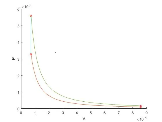
This is the correct plot of the Otto cycle.
RESULT:-
The proper inputs give the accurate plot of the Otto cycle. The value of thermal efficiency comes out to be 0.6299 or 62.99%.