Optimization Using Genetic Algorithm in MATLAB

AIM:- Optimization using Genetic Algorithm in MATLAB

THEORY:-

1)Mathematical Optimization:-It is the selection of a best element (with regard to some criterion) from some set of available alternatives. Optimization problems of sorts arise in all quantitative disciplines from computer science and engineering to operations research and economics.

An optimizationproblem consists of maximizing and minimizing a real function by systematically choosing inout values from within an allowed set and computing the value of the function.

Graph of a given by z = f(x, y) = −(x² + y²) + 4. The global maximum at (x, y, z) = (0, 0, 4) is indicated by a blue dot.

2) Genetic Algorithm(GA):- It is a mathematical model that helps us generate local minimas and maximas. Genetic Algorithm (GA) is a search-based optimization technique based on the principles of Genetics and Natural Selection. It is frequently used to find optimal or near-optimal solutions. It is frequently used to solve optimization problems, in research, and in machine learning.

Flowchart to use GA to find the optimal solution:-

CODE:-

a)For stalagmite function:-

%STALAGMITE FUNCTION DEFINATION

function [F] =stalagmite(input_vector)
f_1x=(sin((5.1*pi).*input_vector(1))+0.5)^6
f_1y=(sin((5.1*pi).*input_vector(2))+0.5)^6

f_2x=exp(-4*log(2)*(((input_vector(1)-0.0667)^2)/(0.64)));
f_2y=exp(-4*log(2)*(((input_vector(2)-0.0667)^2)/(0.64)));

f=f_1x*f_2x*f_1y*f_2y;
[F]=-f
end

Explanation:-

Here, we define a new function called 'Stalagmite', in which we define are formula for calculating our result.

Formula:-

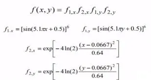
For calculating the maxima of a fucntion we need to multiply the function with '-1' as the function for ga in its own form calculates the minima.

b)Main code:-

%Optimization Using Genetic Algorithm
clear all
close all
clc

%Input
x=linspace(0,0.6,150);
y=linspace(0,0.6,150);
iterations=25;

%Creating a 2D Array

[xx yy]=meshgrid(x,y);

%Computation Of Stalagmite Function
for i=1:length(xx)
for j=1:length(yy)
    input_vector(1)=xx(i,j);
    input_vector(2)=yy(i,j);
  f(i,j)=stalagmite(input_vector);
end
end

%Unbounded
tic
for i=1:iterations
    [inputs,fopt(i)]=ga(@stalagmite,2);
    xopt(i)=inputs(1);
    yopt(i)=inputs(2);
end
Case_1=toc

figure(1)
subplot(2,1,1)
hold on
surfc(x,y,-f)
shading interp
plot3(xopt,yopt,fopt,'marker','o','markersize',5,'markerfacecolor','r');
title('Unbounded');
subplot(2,1,2)
plot(fopt)
xlabel('Iterations')
ylabel('Maxima')

%Bounded
tic
for i=1:iterations
    [inputs,fopt(i)]=ga(@stalagmite,2,[],[],[],[],[0;0],[1;1]);
    xopt(i)=inputs(1);
    yopt(i)=inputs(2);
end
Case_2=toc

figure(2)
subplot(2,1,1)
hold on
surfc(x,y,-f)
shading interp
plot3(xopt,yopt,fopt,'marker','o','markersize',5,'markerfacecolor','r');
title('Bounded');
subplot(2,1,2)
plot(fopt)
xlabel('Iterations')
ylabel('Maxima')

%Increase in population size

options=optimoptions('ga');
options=optimoptions(options,'PopulationSize',170);

tic
for i=1:iterations
    [inputs,fopt(i)]=ga(@stalagmite,2,[],[],[],[],[0;0],[1;1],[],[],options);
    xopt(i)=inputs(1);
    yopt(i)=inputs(2);
end

Case_3=toc

figure(3)
subplot(2,1,1)
hold on
surfc(x,y,-f)
shading interp
plot3(xopt,yopt,fopt,'marker','o','markersize',5,'markerfacecolor','r');
title('Bounded with Icrease in Population Size');
subplot(2,1,2)
plot(fopt)
xlabel('Iterations')
ylabel('Maxima')

Explanation:-

1) Linspace command is used to define the no. of input variables.

2)Meshgrid command is used to create a 2D array. We use the for loop to calculate the values of the stalagmite fucntion.

3)For loop is used to create an input vector of the outputs.

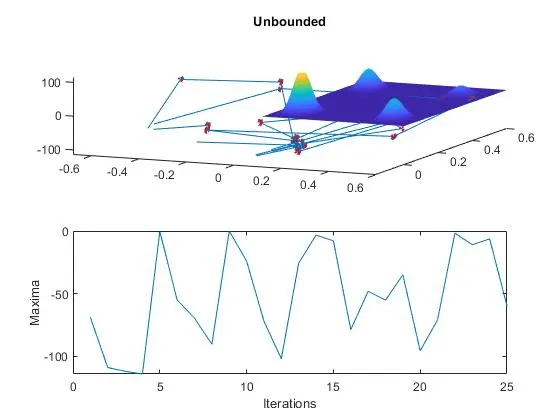
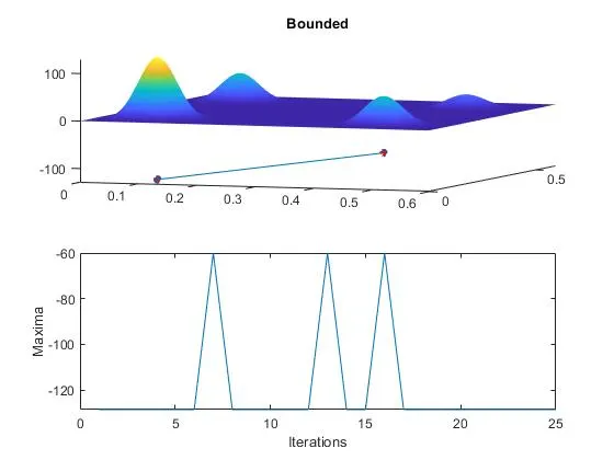
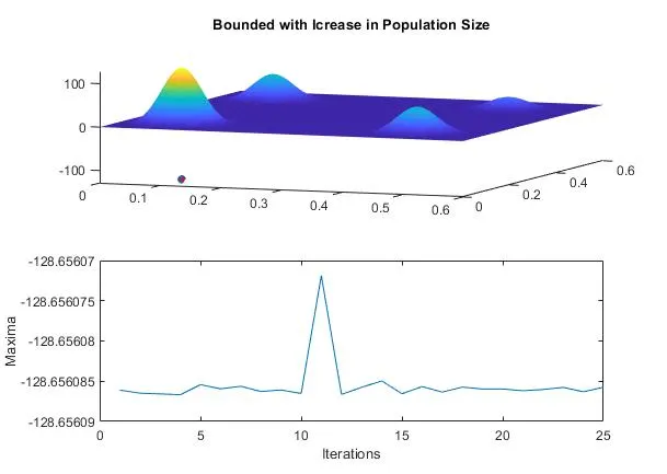
For unbounded:-

x = ga(fun,nvars,A,b,Aeq,beq,lb,ub)

In this synatx we put the function and the no. of variables. Apart for that we also have to put the values for the remaining inputs. Since, we only need lb and ub, we put those values and in place of the remaining values we put an empty matrix('[]').

For bounded with increase in population size:-

x = ga(fun,nvars,A,b,[],[],lb,ub,nonlcon,IntCon,options)

In this synatx we put the function and the no. of variables. Apart for that we also have to put the values for the remaining inputs. Since, we only need lb and ub, we put those values and in place of the remaining values we put an empty matrix('[]'). Here, we also uitlize the options command.Options are a way of combining a set of name-value pairs. They are useful because they allow you to: Tune or modify the optimization process. Select extra features, such as output functions and plot functions.

Optimoptions:-This MATLAB function returns a set of default options for the SolverName solver.

A,b are linear inequality constraints.

Aeq,Beq are linear equality constraints.

lb is lower bound.

ub is upper bound.

plot3 command is used to plot 3D plots.

surfc command is used to plot contour from the values of the meshgrid.

subplot is used to plot more than 1 graph in a figure.

nonlcon is a function that accepts a vector or array and returns two arrays.

IntCon is a vector of positive integers that contains the x components that are integer-valued.

xlabel is used to name the x axis

ylabel is used to name the y axis.

title is used to give title of the figure.

OUTPUT:-

We get the plots for all the 3 cases:

CASE 1:- Unbounded

CASE 2:- Bounded

CASE 3:- Bounded with Increase in Population Size

Time stamps:-

>> Case_1

Case_1 =

   61.1845

>> Case_2

Case_2 =

   45.2599

>> Case_3

Case_3 =

  144.8389

Value of Output fopt(i):-

fopt(i)

ans =

 -128.6561​

RESULT:-

From this program we can understand the concept of genetic algorithm and undertsand the stalagmite function and ways to optimise it.

REFERENCES:-

[1] https://in.mathworks.com/help/gads/ga.html#:~:text=ga%20evaluates%20the%20matrix%20product%20Aeq*x%20as%20if%20x,if%20no%20linear%20equalities%20exist.)

[2] https://skill-lync.freshdesk.com/support/solutions/articles/43000584189-genetic-algorithm-explained-

[3] https://en.wikipedia.org/wiki/Mathematical_optimization