Literature review : RANS derivation and analysis

RANS DERIVATION AND ANALYSIS

AIM:

1. Applying Reynolds’s decomposition to the NS equation and getting the Reynolds’s stress expression
2. Understanding the term of Reynolds’s stress
3. What is Turbulent Viscosity and differentiating from Molecular Viscosity

INTRODUCTION:

REYNOLD’S DECOMPOSITION TO THE NS EQUATION:

In fluid dynamics and turbulence theory, Reynolds Decomposition is a mathematical technique used to separate the expectation value of a quantity from its fluctuations. For example, for a quantity υ the decomposition would be,

Where denotes the expectation value of u and uʹ, are the deviations from the expectation value. The fluctuations are defined as the expectation value subtracted from quantity u such that their time average equals to zero.

The expected value , is often found from an ensemble average which is an average taken over multiple experiments under identical conditions. The expected value is also sometimes denoted (u), but it is also often seen with over-bar notation.

Direct numerical simulation or Navier-Strokes equations completely in (x.y.z,t) is only possible on small computational grids and small time step when Reynolds numbers are low. Due to computational constraints, simplifications of Navier-Stokes equations are useful to parameterize turbulence that is smaller than computational grid, allowing larger computational domains.

Reynolds decomposition allows the simplification the Navier-Strokes equation by substituting in the sum of the steady component and perturbations to the velocity profile and taking the mean value. The resulting equation contains a nonlinear term known as Reynolds stress which gives rise to turbulence.

REYNOLDS AVERAGED NAVIER-STROKES EQUATIONS:

By hand of a time averaging of the NS equations and the continuity equations for incompressible fluids, the basic equations for the averaged turbulent flow will be derived in the following. The flow field can then be described only with the help of the mean values.

In order to be able to take a time average, the momentary value is decomposed into the parts mean value and fluctuating value.

The momentary velocity components is u , the time averaged value is named and the fluctuating velocity has the letter uʹ. With help of this definition the decomposition can mathematically be written as:

...................................................................................................................................................................... Eq.1-1

Analogously for the density and the temperature:

..................................................................................................................................................................................................Eq.1-2

Which will however be considered constant in the following.

The chosen average method takes the mean value at a fix place in space and averaged over a time span that is large enough for the mean values to be independent of it.

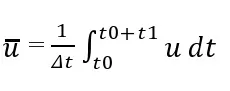......................................................................................................................................................................................................................Eq.1-3

The time averaged values of the fluctuating value are defined to be zero:

Firstly the continuity equation is averaged. If we substitute the expressions of the velocities from Eq.1-1 into the continuity equation we get:

...........................................................................................................................................................................Eq.1-4

The time average of the last equation is written as:

...............................................................................................................................................................Eq.1-5

Before we look at the transformation and reduction of Eq.1-5, a summary of rules for time average shall be given:

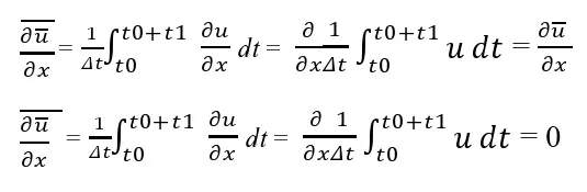......................................................................................................................................................................Eq.1-6

....................................................................................................................................................Eq.1-7

The averaged derivatives of the fluctuations are also zero according to these rules, so that the time averaged continuity equation is:

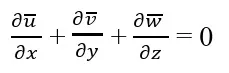........................................................................................................................................................................................................................Eq.1-8

Now the NS equations will be time averaged. The average will be exemplified for the x-component. Beforehand a small transformation of the advection term from continuity equation:

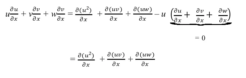...........................................................................................................................................Eq.1-9

The expression for the decomposition of the velocities from the Eq.1-1 is now substituted into the transformed Navier-Strokes equation and a time average is done:

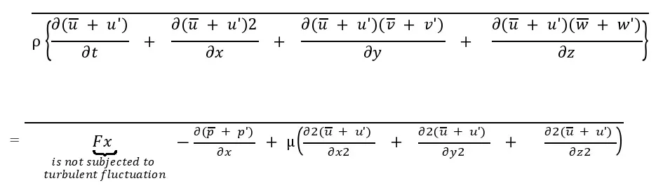.....................................................................................................................Eq.1-10

Application of the rules from the Eq.1-6 and Eq.1-7 shows that among others the terms 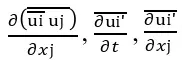from the equation above can be reduced and the equation can be transformed to:

.....................................................................................................................................Eq.1-11

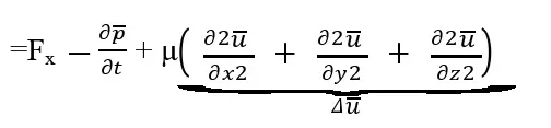
Further small transformation, for example a repeated application of the product rule and the continuity equation to the advection term, lead to a form of the time averaged NS equations for all three dimensions as:

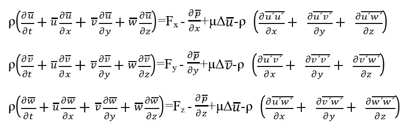..................................................................................................Eq.1-12

Or in tensor form:

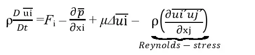............................................................................................................................................................................Eq.1-13

From now on the time averaged fields will not be over lined anymore. So for example u stands for the time averaged velocity component in direction of the x-axis.

We pay attention to the last two terms of the right side of Eq.1-13:

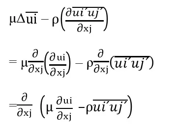..................................................................................................................................................................................................Eq.1-14

The expression in the brackets above corresponds to the total shear stress:

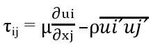.......................................................................................................................................................................................................................Eq.1-15

If we compare to the Navier Strokes equations, it is conspicuous that besides the viscous part an additional term has been added to the total shear stress. This term results from the time average and is generally the dominant part of the total shear stress. Since the term only appears due to the Reynolds average, it is called Reynolds stress or apparent turbulent shear stress. As stated in the introduction to the RANS approach, to lead to the closure of the equation system, an approximation for the Reynolds stresses has to be done, which sets in the relation the apparent shear stresses with the velocity field of the average flow.

TURBULENT VISCOSITY:

Turbulence modelling is the construction and use of a mathematical model to predict the effects of turbulence. The equations governing turbulent flows can only be solved directly for simple case of flow. For most real life turbulent flows, CFD simulations use turbulent models to predict the evolution of turbulence. These turbulent models are simplified constitutive equations that predict the statistical evolution of turbulent flows.

CONCLUSION:

So, the Reynolds Decomposition has been applied to the NS equation and the Reynolds stress was resulted in the equation.