Conjugate Heat Transfer Simulation
SIMULATION OF CONJUGATE HEAT TRANSFER
AIM:
To simulate the conjugate heat transfer through a pipe using converge and analyse the results with three different mesh grids and three different super-cycle stage intervals.
OBJECTIVES:
The term conjugate heat transfer is used to describe the process which involves variations of temperature within solids and fluids, due to thermal interaction between the solids and fluids. The exchange of thermal energy between the two physical bodies is called study of Heat Transfer. The rate of transferred heat is directly proportional to the temperature difference of the bodies.
Conjugate heat transfer corresponds with the combination of heat transfer in solids and heat transfer in fluids. In solids, conduction often dominates whereas in fluids convection usually dominates.
GEOMETRY:
A hollow pipe is created with inner radius 0.015m, outer radius 0.02m and length 0.2m.
INT VELOCITY CALCULATION:
Re = ρ . V. D
μ
For Re= 7000 and Temp= 300K,
7000= 1.185 (kg/m3).V.0.03 (m)
1.85x10⁻⁵ (kg/m-s)
V= 3.64m/s
CASE SETUP:
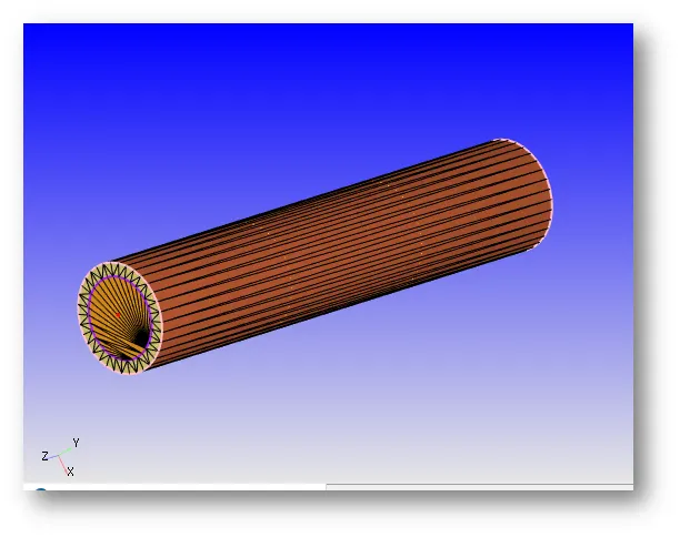
Here for the simulation process, the air is selected for fluid region and aluminium is selected for solid region. In run parameters, solver is selected as transient with time based simulation type. Full hydrodynamic is chosen for the simulation mode and the gas flow solver is compressible.
In simulation time parameter:
End time: 0.5sec
Initial time-step: 1e-07sec
Min time-step: 1e-07sec
Max time-step: 1.0sec
In boundary condition:
Inlet (BOUNDARY ID-3): Pressure- Zero Normal Gradient
Velocity- 3.64m/s (as per calculation)
Temperature- 300K
Outlet (BOUNDARY ID-4): Pressure- 101325Pa
Velocity- Zero Normal Gradient
Solid Outer Wall: Wall motion type- Stationary
Surface movement- Fixed
Temperature-Heat flux- (-) 1000W/m2
Solid Side: Wall motion type- Stationary
Surface movement- Fixed
Temperature- Zero Normal Gradient
Interface: This boundary separates the two types of material or phases
Wall motion type- Stationary
Fluid region is selected in forward side and Solid region is selected in reverse side.
Forward side: Temperature- Law of wall
Velocity- Law of wall
Reverse side: Temperature- Specified value
Velocity- Slip
Turbulence modelling- RNG k-ε
In super-cycle modelling:
In this method, initially both fluid and solid has been solved together using transient solver and at a particular time the fluid solver get freezes. During this, solid is being solved till it reaches the steady state and then unfreezes the fluid solver. This process is repeated until it gets converged.
The super-cycle stage has been set with three different intervals- 0.01, 0.02, 0.03sec respectively.
In grid control:
The base grid also has been set with three different mesh grids- 4e-3, 3e-3, 2e-3m respectively.
MESH:
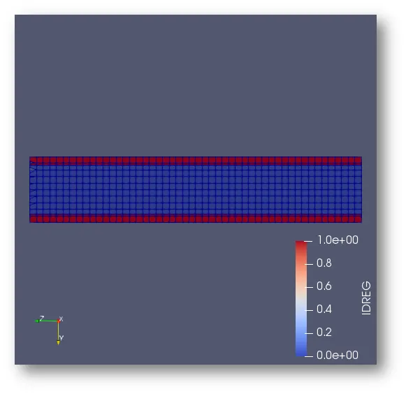
Mesh-1: 4e-3m
Surface with edges in IDREG:
Temperature:
Temperature contours: https://www.youtube.com/watch?v=rayh8UOE5nQ&feature=youtu.be
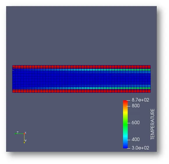
When the simulation starts, the solid region slowly gets heated up and at a particular point of time it reaches the max temp of 870K. As it does the fluid also gets heated and reaches at 300K then it remains at steady state till simulation gets over.
Velocity:
Velocity contours: https://www.youtube.com/watch?v=lvfEw7q0JWY&feature=youtu.be
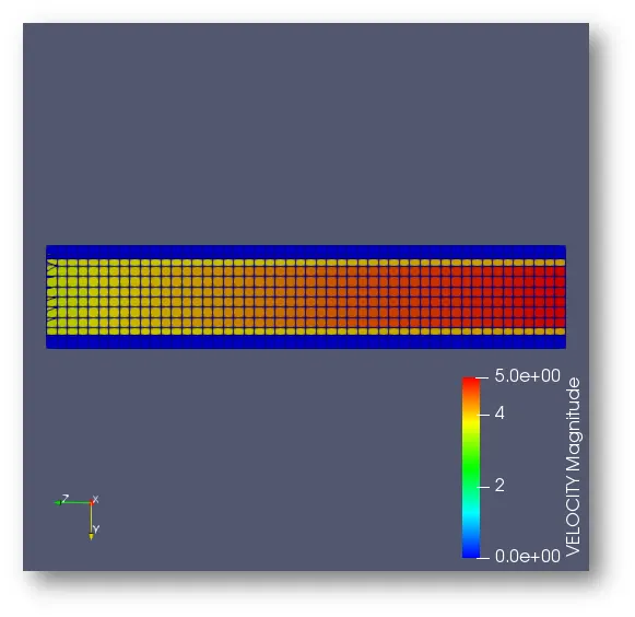
It is assumed that the velocity of the fluid is zero at the wall region and at the inlet, the initial velocity will be 3.64m/s and as it move towards the outlet port the velocity gets increased to 5m/s since the pressure gets decreased.
Y+:
y+ contours: https://www.youtube.com/watch?v=ew6QV_89v9s&feature=youtu.be
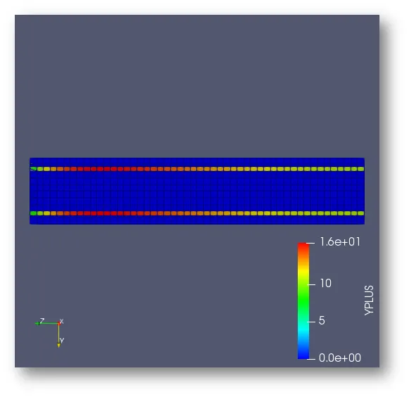
The y+ value is a non dimensional term that can be used to understand how coarse or fine our grid is. In this mesh grid, y+ value is 16 which is gretaer than 10 so it comes under turbulent region.
Mesh-2: 3e-3m
Surface with edges in IDREG:
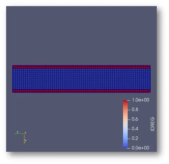
Temperature:
Temperature contours: https://www.youtube.com/watch?v=EbVviPPsSOE&feature=youtu.be
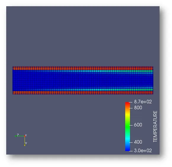
When the simulation starts, the solid region slowly gets heated up and at a particular point of time it reaches the max temp of 870K. As it does the fluid also gets heated and reaches at 300K then it remains at steady state till simulation gets over.
Velocity:
Velocity contours: https://www.youtube.com/watch?v=r6XNxhtUlpI&feature=youtu.be
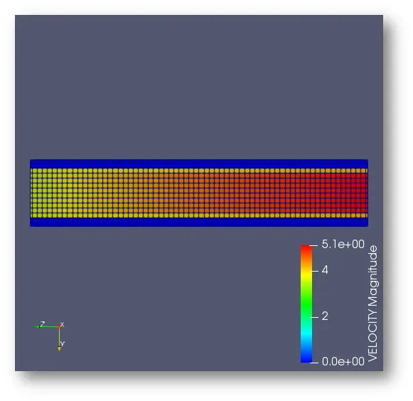
It is assumed that the velocity of the fluid is zero at the wall region and at the inlet, the initial velocity will be 3.64m/s and as it move towards the outlet port the velocity gets increased to 5.1m/s since the pressure gets decreased.
Y+:
Y+ contours: https://www.youtube.com/watch?v=mHzfPIHd2XQ&feature=youtu.be
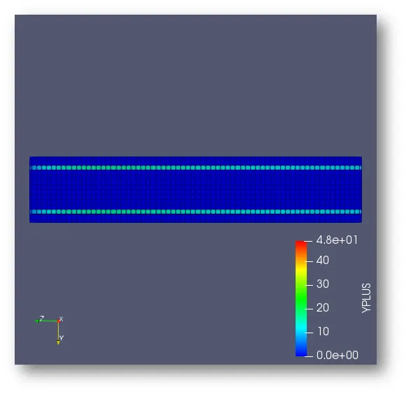
The y+ value is a non dimensional term that can be used to understand how coarse or fine our grid is. In this mesh grid, y+ value is greater than or equal to 10 so it comes under turbulent region.
Mesh-2: 2e-3m
Surface with edges in IDREG:
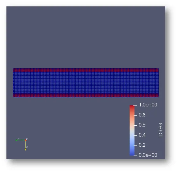
Temperature:
Temperature contours: https://www.youtube.com/watch?v=4tnAT8Mx0qs&feature=youtu.be
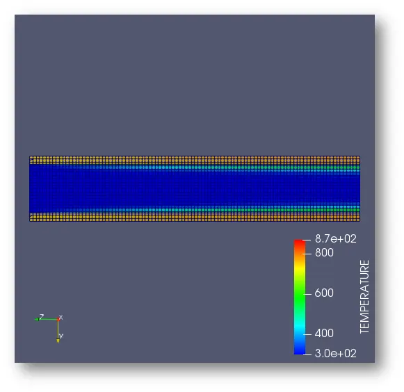
When the simulation starts, the solid region slowly gets heated up and at a particular point of time it reaches a temp of less than or equal to 800K. As it does the fluid also gets heated and reaches at 300K then it remains at steady state till simulation gets over.
Velocity:
Velocity contours: https://www.youtube.com/watch?v=oVWSQkLIdo8&feature=youtu.be
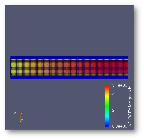
It is assumed that the velocity of the fluid is zero at the wall region and at the inlet, the initial velocity will be 3.64m/s and as it move towards the outlet port the velocity gets increased to 5.1m/s since the pressure gets decreased.
Y+:
Y+ contours: https://www.youtube.com/watch?v=gTsI5T86EJ4&feature=youtu.be
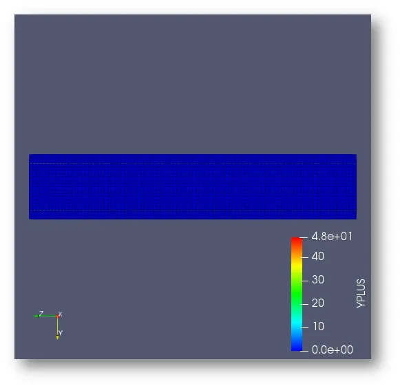
The y+ value is a non dimensional term that can be used to understand how coarse or fine our grid is. In this mesh grid, y+ value is less than 10 so it comes under viscious sub layer region.
Mean Temperatue of Fluid Region:
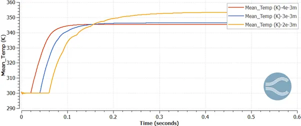
As you can see from the above graph, when the mesh size is decreased the steady state mean temperature value in the fluid region gets increased.
Mean Temperature of Solid Region:
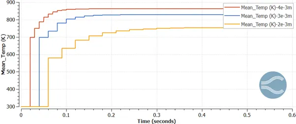
When it comes to solid region it is the vice versa of the mean temperature of fluid region, i.e. when the mesh size is decreased the mean temperature of solid region also gets decreased.
Total Cell Count:
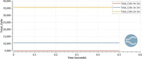
From the above graph, when the mesh grid size is small the total cell count will be higher.
CONCLUSION:
So, the conjugate heat transfer simulation process using converge is done and we have analysed the results based on three different mesh grid size and super-cycle intervals along with Y+ output files for three mesh grids.