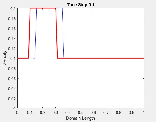
Linear Convection for varying timesteps

Objective:

1. Find Numerical Solution to the One-Dimensional Linear Convection equation.
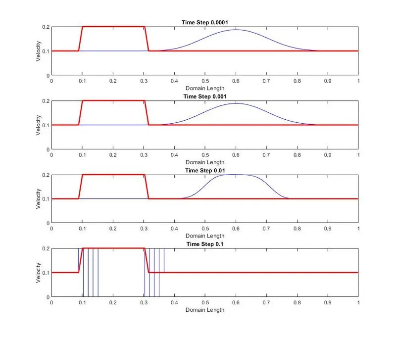
2. Compare the original and final velocity profiles in a single figure window for time steps, dt = 1e-4, 1e-3, 1e-2, and 1e-1
3. Explain the CFL criteria that govern the linear convection equation. Does this criterion apply to an implicit solution as well?
4. From the plots obtained: Explain how the change in time step size affects numerical diffusion, instability, the courant number and accuracy. How does change in time step size affect these phenomena?

Derivation:

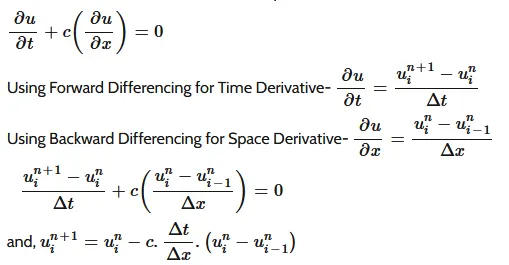
For the solution, we have to use First-Order Forward Differencing for the Time Derivative and First-Order Backward/Rearward Differencing for the space term.

One-Dimensional Linear Convection Equation:

∂u∂t+c(∂u∂x)=0

Using Forward Differencing for Time Derivative- ∂u∂t=un+1i−uniΔt

Using Backward Differencing for Space Derivative- ∂u∂x=uni−uni−1Δx

un+1i−uniΔt+c(uni−uni−1Δx)=0

and, un+1i=uni−c.ΔtΔx.(uni−uni−1)

Here n denotes the Time Step and i denotes the node.

Main Code:

% Week 4.1 - Linear Convection for varying number of nodes

clear all
close all
clc

% Inputs for Linear Convection
L = 1;          % Length in meters
c = 1;          % Constant convection coefficient in meters/second
dt = [1e-4, 1e-3, 1e-2, 1e-1];      % Time step in seconds
t = 0.4;        % Simulation time in seconds

% Number of nodes- to be used 20, 40, 80 and 160
n = 80;

% Node array
x = linspace(0, L, n);
% Element size
dx = L/(n-1);

% Defining the Initial Wave for time t = 1
x_start = 0.1;      % Start value for u=2m/s
x_end = 0.3;        % End value for u=2m/s
n_start = round((x_start/dx)+1);    % Finding starting node
n_end = round((x_end/dx)+1);        % Finding end node

% Initialising arrays and boundary conditions
u = 0.1 * ones(1, n);
u(n_start:n_end) = 0.2;
u_old = u;          % Assinging u to new variable
u_initial = u;

% Total number of time steps
nt = t ./ dt;
% Time Step
for j = 1:4
    tic                     % Starting Stopwatch
    % Time Loop
    for  k=1:nt(j)
            % Space loop
            for i = 2:n
                u(i) = u_old(i) - (c*dt(j)/dx)*(u_old(i)-u_old(i-1));
            end
            u_old = u;         % Assigning u_old with new u values
    end
    time(j) = toc;          % Stopping Stopwatch
    u_old = u_initial;      % Assigning u_old with initial u for next time step
    figure(1)
    subplot(4,1,j)
    plot(x, u, 'b')
    hold on
    plot(x, u_initial, 'r', 'linewidth',2)
    axis([0 1 0 0.2])
    xlabel('Domain Length')
    ylabel('Velocity')
    title("Time Step "+dt(j))
end

figure(2)
names = {'Time Step=1e-4', 'Time Step=1e-3', 'Time Step=1e-2', 'Time Step=1e-1'};
bar(time)
% Using YScale, log to convert Y-Axis sclae to log
% Using xticklabels, names to label bars on X-axis
set(gca,'YScale','log','xticklabel',names)
ylabel('Time')

Output plots:

1. Graph comparing Initial profiles and Final Profiles of the numerical solution for all the dt values.

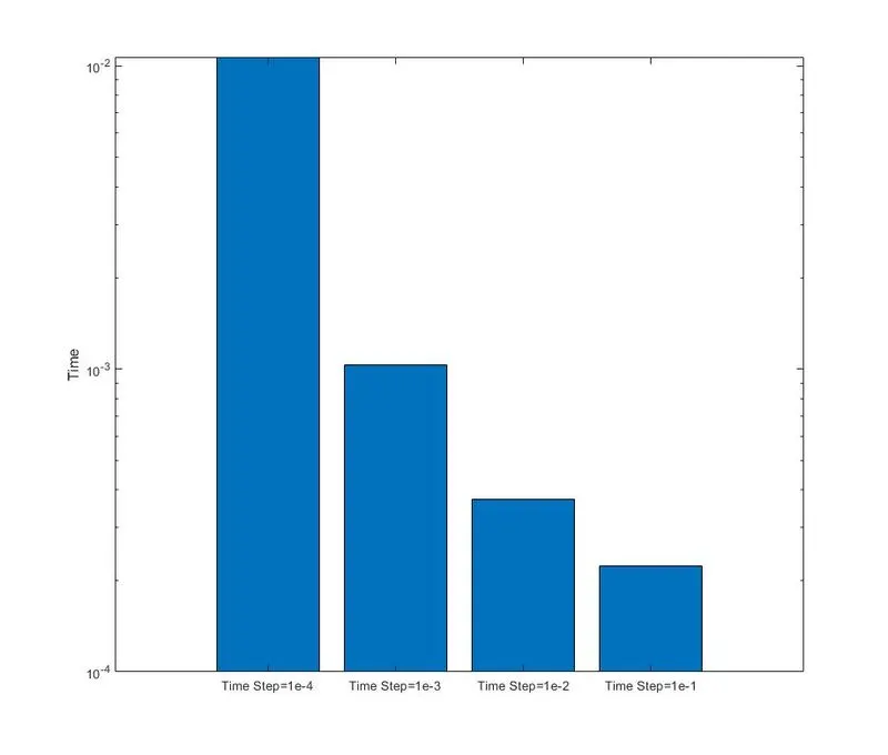
2. Time taken to solve for each time step.

Result Explanation:

It can be seen for Time Step=0.0001 the max output velocity is at about 0.1870m/s, then it goes on increasing to 0.18843m/s for Time Step=0.001 and 0.1999m/s for Time Step=0.01m/s.

But for Time Step=0.1 seconds, due to numerical dispersion, the output is distorted.

Numerical Dispersion:

Dispersion results in a distortion of the propagation of different phases of wave (as seen in the plot of dt=0.1 seconds), which shows up as a wiggle at the start and end of the wave.

This kind of error in solutions occurs due to the approximation in numerical solution (First-Order, Second-Order, etc.)

Numerical Dissipation or Artificial Velocity:

By performing the above operations Numerical Diffusion/Viscosity(Artificial Viscosity) is introduced, which is equal to -

μNUM=c.(ΔxΔ2).(1−c.ΔtΔx)

Here the term, Courant Number

C=c.ΔtΔx

---