Rankine cycle Simulator
OBJECTIVES
- Create a Rankine Cycle Simulator.
- Your code should calculate the state points of the Rankine Cycle based on user inputs.
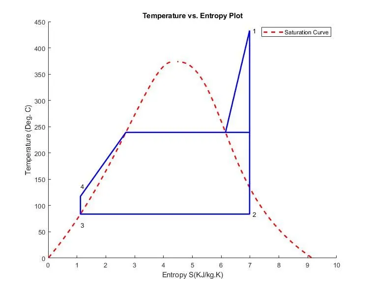
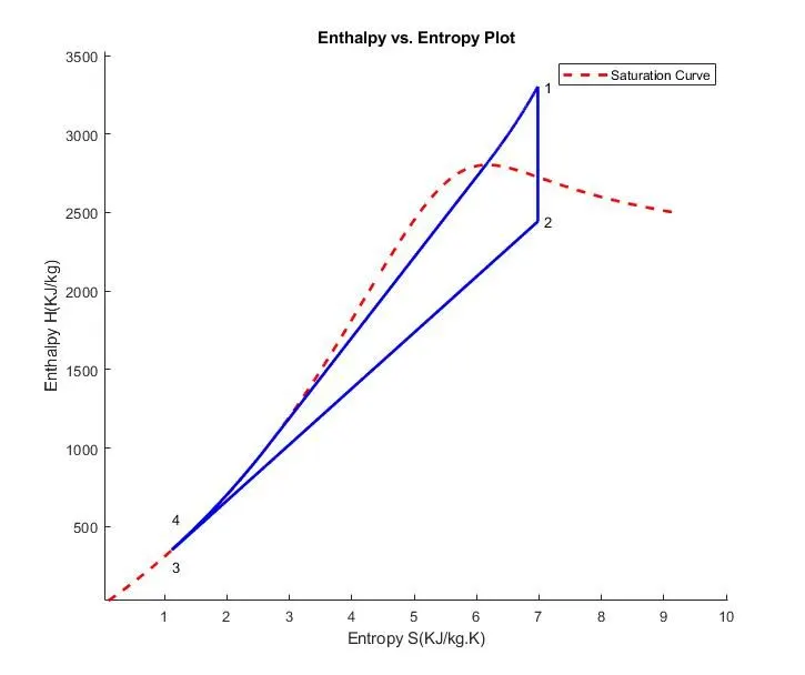
- Then, plot the corresponding T-s and h-s plots for the given set of inputs.
RANKINE CYCLE
The Rankine cycle is an idealized thermodynamic cycle describing the process by which certain heat engines, such as steam turbines or reciprocating steam engines, allow mechanical work to be extracted from a fluid as it moves between a heat source and heat sink.
FOR AN IDEALIZED RANKINE CYCLE
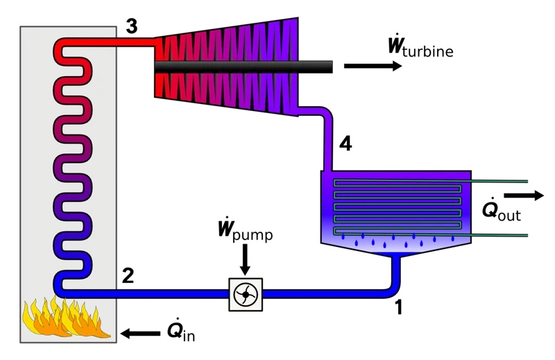
1-2 : The working fluid is pumped from low to high pressure.
2-3 : The high-pressure liquid enters a boiler, where it is heated at constant pressure by an external heat source to become a dry saturated vapour.
3-4 : The dry saturated vapour expands through a turbine, generating power.
CODE
- Code for Displaying Titles and Cycle processes
clear all
close all
clc

% Displaying titles and cycles processes
disp('RANKINE CYCLE');
disp('1-2 is Isentropic Expansion in the Turbine');
disp('2-3 is Const Pressure Heat Rejection by the Condenser');
disp('3-4 is Isentropic Compression in the Pump');
disp('4-1 is Const Pressure Heat Addition by the Boiler');- Code for User Inputs
% User Input Statements
p1 = input('Enter the Pressure at the Turbine Inlet (in bar)= p1 = ');
t1 = input('Enter the Temperature at the Turbine inlet (in Degree Celcius)= t1 = ');
p2 = input('Enter the Pressure at the Condenser (in bar)= p2 = ');- Code for extracting data from XSteam Library
% Extracting data from XSteam.m
% At State Point 1
h1 = XSteam('h_pt', p1, t1);        % Enthalpy
s1 = XSteam('s_pt', p1, t1);        % Entropy
% At State Point 2
s2 = s1;                            % Isentropic Expansion
sf2 = XSteam('sL_p', p2);           % Saturated Liquid Entropy
sg2 = XSteam('sV_p', p2);           % Saturated Vapour Entropy
x2 = (s2-sf2)/(sg2-sf2);
hf2 = XSteam('hL_p', p2);
hg2 = XSteam('hV_p', p2);
h2 = hf2 + (x2*(hg2-hf2));
t2 = XSteam('Tsat_p', p2);
% At State Point 3
p3 = p2;                            % Constant pressure heat rejection
t3 = t2;
s3 = XSteam('sL_p', p3);
h3 = XSteam('hL_p', p3);
% At State Point 4
s4 = s3;
p4 = p1;
cp4 = XSteam('Cp_ps', p4, s4);
cv4 = XSteam('Cv_ps', p4, s4);
k = cp4/cv4;
t4 = t3/((p3/p4)^((k-1)/k));- Calculating Heat, Work and Efficiency values
% Work Done by Turbine
Wt = h1 - h2;

% Work Done for Pump
v3 = XSteam('vL_p', p3);
Wp = v3*(p4-p3)*100;
h4 = h3 + Wp;

% Net Work Done
Wn = Wt - Wp;

% Heat added in the system
Q_add = h1 - h4;

% Heat out of the system
Q_out = h2 - h3;

%Thermal Efficiency
efft = (Wn/Q_add)*100;

%Specific Steam Consumption
SSC = (3600/Wn);            % Mass Flow Rate per Unit Power

% Temperature, Entropy and Enthalpy at the Vapour and Liquid
t6 = XSteam('Tsat_p', p1);
s5 = XSteam('sL_p', p1);
s6 = XSteam('sV_p', p1);
h5 = XSteam('hL_p', p1);
h6 = XSteam('hV_p', p1);
t5=t6;- Plotting Saturation Curve
%Plotting Saturation Curve
t = linspace(1, 375,1000);

for i = 1:length(t)
    sf(i) = XSteam('sL_T', t(i));
    sg(i) = XSteam('sV_T', t(i));
    hf(i) = XSteam('hL_T', t(i));
    hg(i) = XSteam('hV_T', t(i));
end
- Plotting T-s graph
% Plotting T-s Curves
figure(1)
hold on
plot(sf, t, 'r','linewidth',2,'linestyle', '--')
plot(sg, t, 'r','linewidth',2,'linestyle', '--')
plot([s1 s2 s3 s4 s5 s6 s1], [t1 t2 t3 t4 t5 t6 t1],'b','linewidth',2)
% plot([s2 s3], [t2 t3],'b','linewidth',2)
% plot([s3 s4], [t3 t4],'b','linewidth',2)
% plot([s4 s5], [t4 t5],'b','linewidth',2)
% plot([s5 s6], [t5 t6],'b','linewidth',2)
sc1 = linspace(s6, s1, 1000);
for m = 1:length(sc1)
    Tc1(m) = XSteam('T_ps', p1, sc1(1));
end
plot(sc1, Tc1,'b','linewidth',2)
text(s1+0.1, t1, '1')
text(s2+0.1, t2, '2')
text(s3, t3-20, '3')
text(s4, t4+20, '4')
title('Temperature vs. Entropy Plot')
xlabel('Entropy S(KJ/kg.K)')
ylabel('Temperature (Deg. C)')
legend('Saturation Curve')- Plotting H-s graph
% Plotting h-s Curves
figure(2)
hold on
plot(sf, hf, 'r','linewidth',2,'linestyle', '--')
plot(sg, hg, 'r','linewidth',2,'linestyle', '--')
plot([s1 s2], [h1 h2],'b','linewidth',2)
plot([s2 s3], [h2 h3],'b','linewidth',2)
plot([s3 s4], [h3 h4],'b','linewidth',2)
hc = linspace(h4, h5, 100);
for k = 1:length(hc)
    sch(k) = XSteam('s_ph', p1, hc(k));
end
plot(sch, hc,'b','linewidth',2)
plot([s5 s6], [h5 h6],'b','linewidth',2)
for n = 1:length(sc1)
    hc1(n) = XSteam('h_ps', p1, sc1(n));
end
plot(sc1, hc1,'b','linewidth',2)
text(s1+0.1, h1, '1')
text(s2+0.1, h2, '2')
text(s3, h3-100, '3')
text(s4, h4+200, '4')
title('Enthalpy vs. Entropy Plot')
xlabel('Entropy S(KJ/kg.K)')
ylabel('Enthalpy H(KJ/kg)')
legend('Saturation Curve')- Displaying results
% Displaying results
disp('RESULTS');
fprintf('At State Point 1:n');
fprintf('p1: %8.3f bar n', p1);
fprintf('t1: %8.3f C n', t1);
fprintf('h1: %8.3f KJ/kg n', h1);
fprintf('s1: %8.3f KJ/kg.K n ', s1);

fprintf('nAt State Point 2:n');
fprintf('p2: %8.3f bar n', p2);
fprintf('t2: %8.3f C n', t2);
fprintf('h2: %8.3f KJ/kg n', h2);
fprintf('s2: %8.3f KJ/kg.K n', s2);
fprintf('x2: %8.3f  n', x2);

fprintf('nAt State Point 3:n');
fprintf('p3: %8.3f bar n', p3);
fprintf('t3: %8.3f C n', t3);
fprintf('h3: %8.3f KJ/kg n', h3);
fprintf('s3: %8.3f KJ/kg.K n', s3);

fprintf('nAt State Point 4:n');
fprintf('p4: %8.3f bar n', p4);
fprintf('t4: %8.3f C n', t4);
fprintf('h4: %8.3f KJ/kg n', h4);
fprintf('s4: %8.3f KJ/kg.K n', s4);

fprintf('nTurbine Work: %8.3f KJ/kg n', Wt);
fprintf('Pump Work: %8.3f KJ/kg n', Wp);
fprintf('Wnet: %8.3f KJ/kg n', Wn);
fprintf('Efficiency: %8.3f Percent n', efft);
fprintf('SSC: 58.3f KJ/KWh', SSC);
PLOTS
RESULTS
RANKINE CYCLE
1-2 is Isentropic Expansion in the Turbine
2-3 is Const Pressure Heat Rejection by the Condenser
3-4 is Isentropic Compression in the Pump
4-1 is Const Pressure Heat Addition by the Boiler
Enter the Pressure at the Turbine Inlet (in bar)= p1 = 33
Enter the Temperature at the Turbine inlet (in Degree Celcius)= t1 = 433
Enter the Pressure at the Condenser (in bar)= p2 = 0.55
RESULTS
At State Point 1:
p1:   33.000 bar
t1:  433.000 C
h1: 3301.972 KJ/kg
s1:    6.983 KJ/kg.K

At State Point 2:
p2:    0.550 bar
t2:   83.709 C
h2: 2443.092 KJ/kg
s2:    6.983 KJ/kg.K
x2:    0.910

At State Point 3:
p3:    0.550 bar
t3:   83.709 C
h3:  350.523 KJ/kg
s3:    1.119 KJ/kg.K

At State Point 4:
p4:   33.000 bar
t4:  117.523 C
h4:  353.870 KJ/kg
s4:    1.119 KJ/kg.K

Turbine Work:  858.880 KJ/kg
Pump Work:    3.347 KJ/kg
Wnet:  855.533 KJ/kg
Efficiency:   29.020 Percent
SSC: 58.3f KJ/KWh
REFERENCES