Deriving 4th order approximation of a 2nd order derivative using Taylor Table method

CHALLENGE OBJECTIVE:

I. Derive the following 4th order approximations of the second-order derivative.

1. Central difference

2. Skewed right-sided difference

3. Skewed left-sided difference

Prove these skewed schemes are fourth-order accurate.

II. Write a program in Matlab to evaluate the second-order derivative of the analytical function exp(x).cos(x), and compare it with the 3 numerical approximations previously derived.

III. Provide a plot that compares the absolute error between the above-mentioned schemes.

Derivation of the 4th order approximations of the second-order derivative:

1. Central Difference:

The number of nodes required for Central Difference can be found by the following equation,

(Order of accuracy) = (Number of nodes) – (Order of derivative) + 1

Here, Order of accuracy = 4; Order of derivative = 2

Therefore, Number of nodes = 5.

In central difference, we have an equal number of nodes on either side of the point of focus, as shown in the figure of stencil below,

Now for function ‘u’, by Taylor’s Table method, second-order derivative can be evaluated as

`(d^2u)/dx^2 = a.f(i-2)+b.f(i-1)+cf(i)+d.f(i+1)+e.f(i+2)`

Taylor’s table:

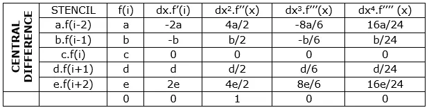
A set of five linear equations can be obtained from the above equation. They can be converted into matrices in the form as A.X=B. Where X(Matrix containing variables a, b, c, d, e) can be solved using Matlab with Matrix Inversion Method.

A.X = B

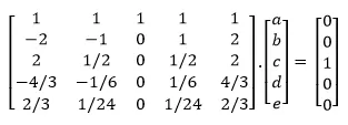
Solving for X in Matlab,

>> A = [ 1 1 1 1 1; -2 -1 0 1 2; 2 1/2 0 1/2 2; -4/3 -1/6 0 1/6 4/3; 2/3 1/24 0 1/24 2/3];
>> B = [0; 0; 1; 0; 0];
>> X = inv(A)*B

X =

   -0.0833
    1.3333
   -2.5000
    1.3333
   -0.0833

a=-0.0833; b=1.3333; c=-2.5000; d=1.3333; e=-0.0833

Therefore we get,

`(d^2u)/dx^2 = (-0.0833.f(i-2)+1.3333.f(i-1)-2.5000f(i)+1.3333.f(i+1)-0.0833.f(i+2))/(dx^2)`

2. Skewed right-sided difference:

The number of nodes required for Skewed right-sided difference can be found by the following equation,

(Order of accuracy) = (Number of nodes) – (Order of derivative)

Here, Order of accuracy = 4; Order of derivative = 2

Therefore, Number of nodes = 6.

Now for function ‘u’, by Taylor’s Table method, the second-order derivative can be evaluated as

`(d^2u)/(dx^2)=a.f(i)+b.f(i+1)+c.f(i+2)+d.f(i+3)+e.f(i+4)+f.f(i+5)`

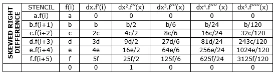
A set of six linear equations can be obtained from the above equation. They can be converted into matrices in the form as A.X=B. Where X(Matrix containing variables a, b, c, d, e, f) can be solved using Matlab with Matrix Inversion Method.

A.X = B

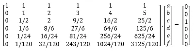
Solving for X in Matlab,

>> A = [1 1 1 1 1 1; 0 1 2 3 4 5; 0 1/2 2 9/2 16/2 25/2; 0 1/6 8/6 27/6 64/6 125/6;0 1/24 16/24 81/24 256/24 625/24; 0 1/120 32/120 243/120 1024/120 3125/120];
>> B = [0; 0; 1; 0; 0; 0];
>> X = inv(A)*B

X =

    3.7500
  -12.8333
   17.8333
  -13.0000
    5.0833
   -0.8333

a=3.7500; b=-12.8333; c=17.8333; d=-13.0000; e=5.0833; f=-0.8333

Therefore, we get,

`(d^2u)/(dx^2)=(3.7500.f(i)-12.8333.f(i+1)+17.8333.f(i+2)-13.0000.f(i+3)+5.0833.f(i+4)-0.8333.f(i+5))/(dx^2)`

3. Skewed left-sided difference:

The number of nodes required for Skewed left-sided difference can be found by the following equation,

(Order of accuracy) = (Number of nodes) – (Order of derivative)

Here, Order of accuracy = 4; Order of derivative = 2

Therefore, Number of nodes = 6.

Now for function ‘u’, by Taylor’s Table method, the second-order derivative can be evaluated as

`(d^2u)/(dx^2)=a.f(i-5)+b.f(i-4)+c.f(i-3)+d.f(i-2)+e.f(i-1)+f.f(i)`

Taylor’s table:

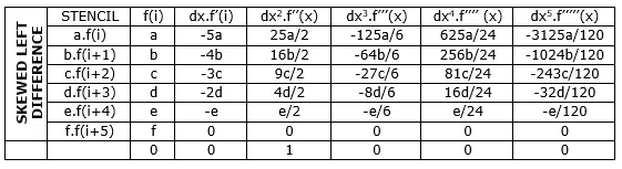
A set of six linear equations can be obtained from the above equation. They can be converted into matrices in the form as A.X=B. Where X(Matrix containing variables a, b, c, d, e, f) can be solved using Matlab with Matrix Inversion Method.

A.X = B

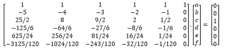
Solving for X in Matlab,

>> A = [1 1 1 1 1 1;-5 -4 -3 -2 -1 0;25/2 8 9/2 2 1/2 0; -125/6 -64/6 -27/6 -8/6 -1/6 0;625/24 256/24 81/24 16/24 1/24 0;-3125/120 -1024/120 -243/120 -32/120 -1/120 0];
>> B = [0; 0; 1; 0; 0; 0];
>> X = inv(A)*B

X =

   -0.8333
    5.0833
  -13.0000
   17.8333
  -12.8333
    3.7500

a=-0.8333; b=5.0833; c=-13.0000; d=17.8333; e=-12.8333; f=3.7500

Therefore, we get,

`(d^2u)/(dx^2)=(-0.8333.f(i-5)+5.0833.f(i-4)-13.0000.f(i-3)+17.8333.f(i-2)-12.8333.f(i-1)+3.7500.f(i))/(dx^2)`

Comparison between Analytical and Numerical Approximations:

The given equation for comparison:

f(x)=exp(x)*cos(x)

The second derivative of the given equation is:

f''(x)= -2*exp(x)*sin(x)

Let x = pi/4, and have a range for dx – dx varies between pi/500 to pi/5 having 200 elements.

MAIN MATLAB CODE:

clear all
close all
clc

% The given eqaution: f(x)=exp(x)*cos(x)
% First Derivative: f'(x)=exp(x)*[cos(x)-sin(x)]
% Second Derivative: f''(x)= -2*exp(x)*sin(x)

% Comparing the analytical and numerical approximations for x=pi/4 and dx=pi/500 to pi/5
% Defining input
x = pi/4;
dx = linspace(pi/500, pi/5, 200);

% Calling function analytical_derivation for analytical result
analytical_derivative = analytical_derivation(x);

% Calling function- function_value to allocate values to functions in
% stencil
for i=1:length(dx)
f(i) = function_value(x);
f_1(i) = function_value(x+dx(i));       % Using f for forward difference
f_2(i) = function_value(x+2*dx(i));     % Using f for forward difference
f_3(i) = function_value(x+3*dx(i));     % Using f for forward difference
f_4(i) = function_value(x+4*dx(i));     % Using f for forward difference
f_5(i) = function_value(x+5*dx(i));     % Using f for forward difference
r_1(i) = function_value(x-dx(i));       % Using r for rear difference
r_2(i) = function_value(x-2*dx(i));     % Using r for rear difference
r_3(i) = function_value(x-3*dx(i));     % Using r for rear difference
r_4(i) = function_value(x-4*dx(i));     % Using r for rear difference
r_5(i) = function_value(x-5*dx(i));     % Using r for rear difference
end

% Calling functions for numerical approximations errors
% Passing values of dx and analytical values to find the absolute error
for i=1:length(dx)
central_difference_value(i) = central_approximation(dx(i), r_2(i), r_1(i), f(i), f_1(i), f_2(i));
central_difference_error(i) = abs(central_difference_value(i) - analytical_derivative);
right_skewed_value(i) = right_approximation(dx(i), f(i), f_1(i), f_2(i), f_3(i), f_4(i), f_5(i));
right_skewed_error(i) = abs(right_skewed_value(i) - analytical_derivative);
left_skewed_value(i) = left_approximation(dx(i), r_5(i), r_4(i), r_3(i), r_2(i), r_1(i), f(i));
left_skewed_error(i) = abs(left_skewed_value(i) - analytical_derivative);
end

%Plotting value of analytical and numerical approximations
subplot(2,1,1)
fplot(analytical_derivative,'--')
xlim([pi/400 pi/4])
ylim([-4 -3])
hold on
plot(dx, central_difference_value, 'linewidth', 2, 'color', 'r')
hold on
plot(dx, right_skewed_value, 'linewidth', 2, 'color', 'g')
hold on
plot(dx, left_skewed_value, 'linewidth', 2, 'color', 'b')
title('Analytical Results vs. Numerical Approximations')
legend('Analytical Result','Central Differencing Values', 'Right Skewed Values', 'Left Skewed Values')

% Plotting logaritmic graphs for above derived errrors
subplot(2,1,2)
loglog(dx, central_difference_error, 'linewidth', 2, 'color', 'r')
hold on
loglog(dx, right_skewed_error, 'linewidth', 2, 'color', 'g')
hold on
loglog(dx, left_skewed_error, 'linewidth', 2, 'color', 'b')
title('Numerical Approximations Errors')
legend('Central Differencing Error', 'Right Skewed Error', 'Left Skewed Error')

Code for Analytical Derivation:

function analytical = analytical_derivation(x)
analytical = -2 * exp(x) * sin(x);
end

Code for Function Values:

function value = function_value(x)
value = exp(x)*cos(x);
end

Code for Central Approximation:

function central_value = central_approximation(dx, r_2, r_1, f, f_1, f_2)
% Using Central Differencing
central_value = (-0.0833*r_2 + 1.3333*r_1 - 2.5*f + 1.3333*f_1 - 0.0833*f_2)/(dx^2);

end

Code for Right-Skewed Approximation:

function right_value = right_approximation(dx, f, f_1, f_2, f_3, f_4, f_5)
% Using Right-Skewed Differencing
right_value = (3.75*f - 12.8333*f_1 + 17.8333*f_2 - 13*f_3 + 5.0833*f_4 - 0.8333*f_5)/(dx^2);
end

Code for Left-Skewed Approximation:

function left_value = left_approximation(dx, r_5, r_4, r_3, r_2, r_1, f)
% Using Left-Skewed Differencing
left_value = (-0.8333*r_5 + 5.0833*r_4 - 13*r_3 + 17.8333*r_2 - 12.8333*r_1 + 3.75*f)/(dx^2);
end

Plots:

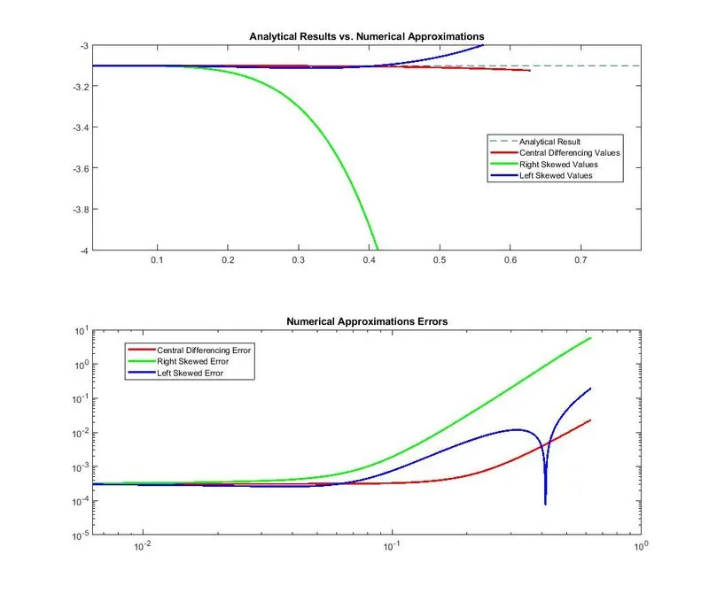
Results:

• From Plot 1(Value Comparision) it can be seen that Central Differencing is a better numerical approximation with less deviation from the analytical result than Right-Skewed and Left-Skewed.
• From Plot 2 (Error Comparision) it can be seen that the Central Differencing maintains lower and more consistent error than Right-Skewed and Left-Skewed errors.

Why Skewed is useful?:

Central Differencing requires an equal number of nodes on both sides of the node that is under evaluation. But at boundary conditions/nodes this is not possible. Here we can employ Right-Skewed or Left-Skewed numerical approximations on boundary nodes, since the skewed scheme requires nodes only on one side of the interested node.