Getting started with Flow Simulation in SolidWorks

Aim : To study the internal flow simulation of a pipe using various inlet Reynolds number

Objective :

- Run a pipe flow simulation with an inlet Reynolds number of 100,1000 and 10,000.

- For each of these cases do the following

1. Place line probes at 95%, 90% and 85% of the pipe length.
2. Compare the normalized velocity profile at each of these locations.
3. Normalize the velocity profile by the inlet velocity.

Introduction

What is CFD? Computational Fluid Dynamics (CFD) is the process of mathematically modeling a physical phenomenon involving fluid flow and solving it numerically using the computational process.

Using CFD, we are able to analyze complex problems involving fluid-fluid, fluid-solid or fluid-gas interaction. Engineering fields where CFD analyses are frequently used are aerodynamics and hydrodynamics, where quantities such as lift and drag or field properties as pressures and velocities are obtained. Moreover this technology can be used in areas such as cavitation prevention, aerospace engineering, HVAC engineering, electronics manufacturing. CFD is used by many industries in their development work to analyse, optimise and verify the performance of designs before prototyping and physical testing the product. This can significanly reduce the development cost as using physical experiments and tests to get essential engineering data for design can be expensive at the same time CFD is also used to accelerate the product development process.

Theory

Reynold Number.The Reynolds number represents the ratio of inertial forces to viscous forces. It is defined as a characteristic length multiplied by a characteristic velocity and divided by the kinematic viscosity.

This dimentionless number helps to predict flow patterns in different fluid flow situations such as Laminar flow or Turbulent flow. It is assumed that a Reynolds number less than or equal to 2000 indicates laminar flow, and a Reynolds number greater than 4000 indicates turbulent flow. At Reynolds numbers between 2000 and 4000, the flow is unstable due to the onset of turbulence. These flows are sometimes referred to as transitional flows.

Reynold Formula

=Reynolds number

=Density of fluid

=Flow speed(velocity)

=Characteristic linear dimension

=Dynamic viscosity of the fluid

Laminar Flow in pipes occurs when a fluid flows in parallel layers, with no disruption between the layers. At low velocities, the fluid tends to flow without lateral mixing, and adjacent layers slide past one another.

Turbulent Flow is a flow regime characterized by chaotic property changes. This includes rapid variation of pressure and flow velocity in space and time.

Simulation setup

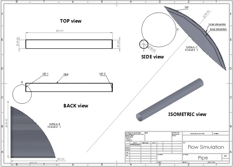
A) Pipe Dimension

Outer diameter : 0.06m

inner diameter : 0.058m

Wall thickness : 0.001m

Length : 0.6m

B) Project Setting

1. Lids are created at both ends of the pipe.
2. Line probes are drawn at the top plane at 85%, 90% and 95% of the pipe length.
3. Choose wizard option in the Flow Simulation tab.

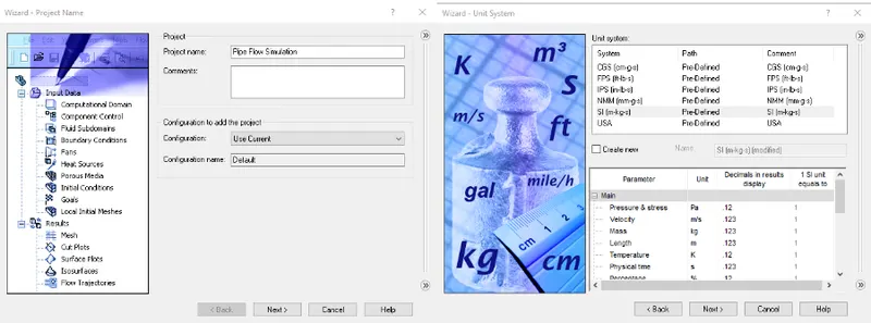
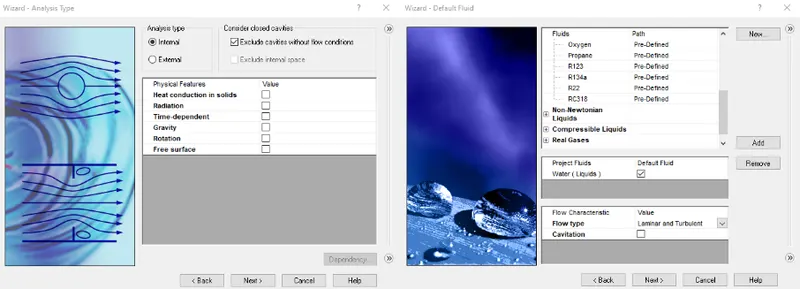
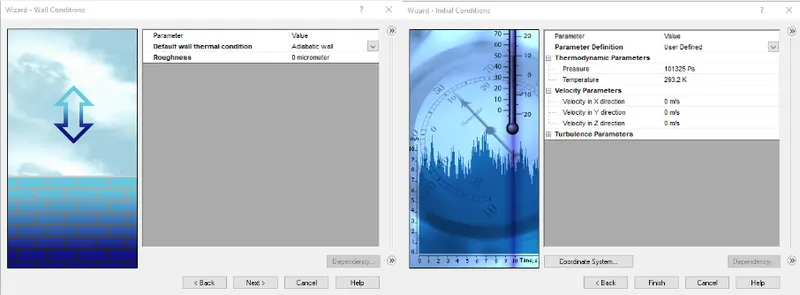
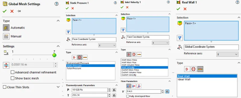
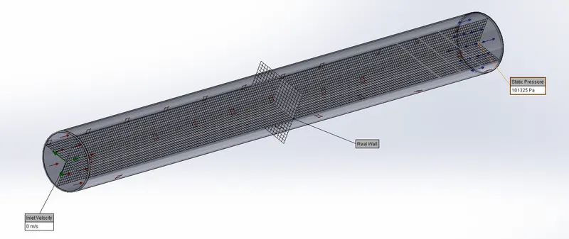
5. Edit the global mesh to the prefered value.

6. Apply boundary condition to the project

- Inlet Velocity : 0m/s

- Static Pressure : 101325Pa

- Wall : Real Wall

7. Apply XY plot and cut plot at each line probes at 85%,90% and 95% to obtain the velocity plot graph and velocity contour graph.

8. Set up a parametric studies with the inlet velocity as an input data and insert the velocity value for the thr reynold number of 100,1000,10000.

9. Choose all the cut plots and XY plots as the output.

10. Run the simulation to obtain all the graphs at once.

RESULT

Case study 1

Reynold Number : 100

100 = (1000 kg/m³ * V * 0.058m) / 8.9*10^-4

V = 0.00153 m/s

Cut plots : 95% 90% 85%

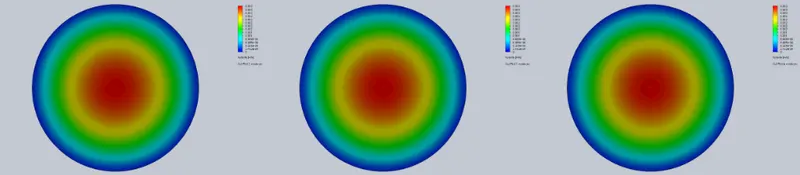
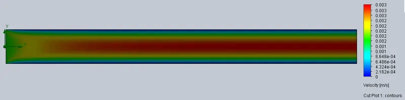
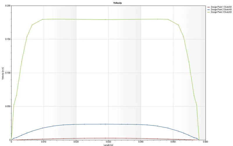
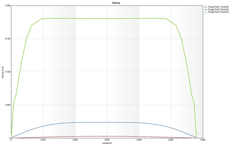
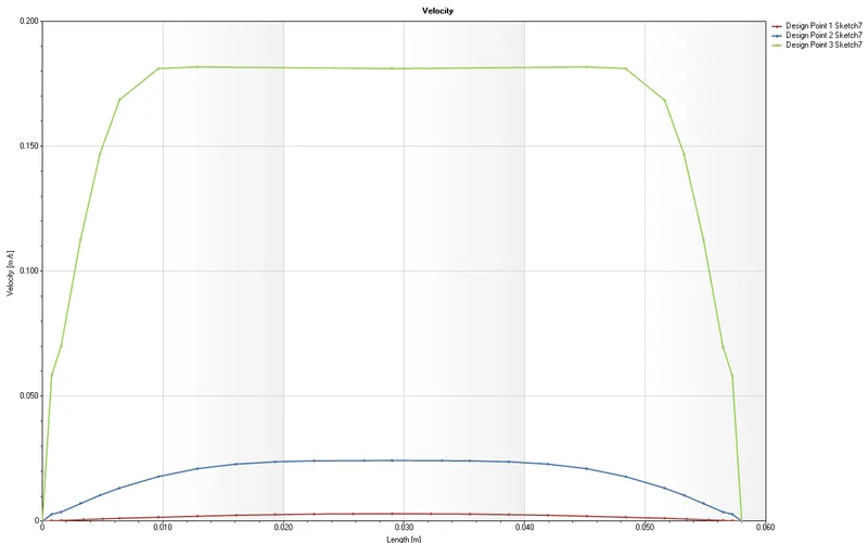
By observing the velocity profile above we can conclude that For Reynold number 100 the flow in the pipe is laminar. The velocity is at maximum at the centre of the pipe (0.003 m/s) and the the velocity is at minimum at he wall of the pipe(0.0002162 m/s).

Case study 2

Reynold Number : 1,000

1000 = (1000 kg/m³ * V * 0.058m) / 8.9*10^-4

V = 0.0153 m/s

Cut plots : 95% 90% 85%

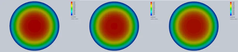
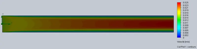
By observing the velocity profile above we can conclude that For Reynold number 1000 the flow in the pipe is laminar. The velocity is at maximum at the centre of the pipe (0.025 m/s) and the the velocity is at minimum at he wall of the pipe(0.002 m/s).

Case study 3

Reynold Number : 10,000

10,000 = (1000 kg/m³ * V * 0.058m) / 8.9*10^-4

V = 0.153 m/s

Cut plots : 95% 90% 85%

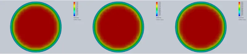
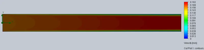
By observing the velocity profile above we can conclude that For Reynold number 10,000 the flow in the pipe is laminar. The velocity is at maximum at the centre of the pipe (0.182 m/s) and the the velocity is at minimum at he wall of the pipe(0.013 m/s).

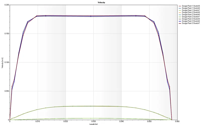
Based on all the cut plots, we can see the velocity contours graph which is influnced by the Reynold Number. It can be stated that the maximum velocity is at the centre of the pipe and the velocity decreases towards the pipe wall. For reynold number 100 the maximum velocity is 0.003 m/s, For reynold number 1000 the maximum velocity is 0.025 m/s For reynold number 10,000 the maximum velocity is 0.128 m/s.

Velocity Plot Graph

Cut plot at 85% (Re : 100, 1000, 10,000 ) (comparison)

Cut plot at 90% (Re : 100, 1000, 10,000 ) (comparison)

Cut plot at 95% (Re : 100, 1000, 10,000 ) (comparison)

Combined Velocity Graph (comparison)

Observation / Conclusion

• In case study 1 & 2 the the velocity contour graphs can be concluded as laminar flow as its Reynold Number are 100 and 1000 respectively. In case study 3 the velocity contour graph shows turbulent flow characteristic as its Reynold Number are 10,000. This proves that Reynold Number <2000 can be considered as laminar flow and Reynold Number >4000 Can be considered as turbulent Flow.
• The velocity at the center of the pipe is high and reduces when moved towards the pipe wall. This can be seen in the velocity contour graph where red color indicates the maximum velocity and blue indicates the minimum velocity.
• The velocity profile at the line probes does not have much difference. this is because the distance between each line probes are close to each other.
• Meshing the pipe at a high level allows the user the obtain more detailed result then meshing at a lower level.