Flow over a cylinder
FLOW SIMULATION OVER A CYLINDER
Using SOLIDWORKS Flow Simulation
AIM: To perform Flow Simulation over a Cylinder of particular Diameter and Length
OBJECTIVE:
- To Perform simulation of a baseline cylinder with external flow and then calculate the Reynolds Number.
- Run a transient flow simulation on a cylinder by increasing the Reynolds number by a factor of 20%, 40%, and 100%
- Calculate the End time of analysis with the help of Domain length and Velocity.
- To obtain the plots for Velocity and Pressure Variations as the Reynolds number is increased.
- Display the flow Simulation Animation
OVERVIEW:
The presence of the fluid viscosity slows down the fluid particles very close to the solid surface and forms a thin slow-moving fluid layer called a boundary layer. The flow velocity is zero at the surface to satisfy the no-slip boundary condition. Inside the boundary layer, flow momentum is quite low since it experiences a strong viscous flow resistance.
The boundary layer flow is sensitive to the external pressure gradient . If the pressure decreses in the direction of the flow, the pressure gradient is said to be favorable.
External flows past objects have been studied extensively because of their many practical applications. For example, airfoils are made into streamline shapes in order to increase the lifts, and at the same time, reducing the aerodynamic drags exerted on the wings.
On the other hand, flow past a blunt body, such as a circular cylinder, usually experiences boundary layer separation and very strong flow oscillations in the wake region behind the body. In certain Reynolds number range, a periodic flow motion will develop in the wake as a result of boundary layer vortice being shed alternatively from either side of the cylinder
The flow past a two-dimensional cylinder is one of the most studied of aerodynamics. It is relevant to many engineering applications. The flow pattern and the drag on a cylinder are functions of the Reynolds number
MODEL GEOMETRY:
Cylinder
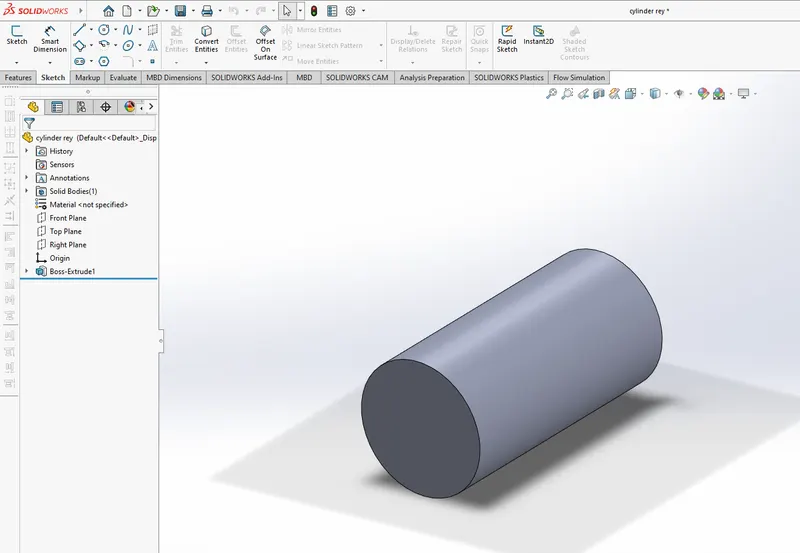
1.Diameter of the Cylinder = 0.05m
2.Length of the Cylinder = 0.1m
CALCULATION:
1.Reynolds Number [Re] Calculation

ρ = Fluid density (kg/m3)
V = Flow or Inlet velocity (m/s)
μ = Dynamic viscosity (pa.s)
L = length or diameter of the fluid (m)
In this case Air is taken as fluid
Therefore,
μ = 1.81 × 10⁻⁵ (pa·s)
ρ = 1.225 kg/m^3
2.Flow and End Time Calculation
Flow Time = Domain Length / Velocity
End Time = 2 * Flow Time
- Domain Length along X axis in this case study is 0.5m
INPUTS BASED ON CALCULATION
For Baseline Calculation
Inlet Velocity = 10 m/s
(Using the Above Formula)
Re= 33839.8
Simulation End Time = 0.1 s
For Re increased by 20%
Inlet Velocity = 12 m/s
(Using the Above Formula)
Re= 40606.8
Simulation End Time = 0.084 s
For Re increased by 40%
Inlet Velocity = 14 m/s
(Using the Above Formula)
Re= 47374.6
Simulation End Time = 0.0714 s
For Re increased by 100%
Inlet Velocity = 20 m/s
(Using the Above Formula)
Re=67679.6
Simulation End Time = 0.05 s
PROCEDURE:
1.After solid modelling of Cylinder is done using the appropriate tool and dimensions. Click on the Flow Simulation tab in Solidworks Interface.
Click on Wizard and provide the following initial condtions given
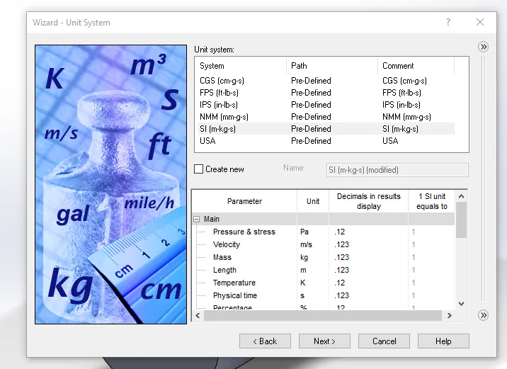
Unit System
Analysis Type
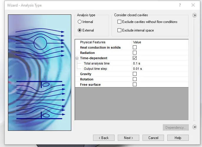
We have given Total Analysis time as 0.1 seconds as it is the End Time for baseline velocity 10 m/s .
Output Time Setup =Total Analysis Time / 10
It can be changed as per the Input data given
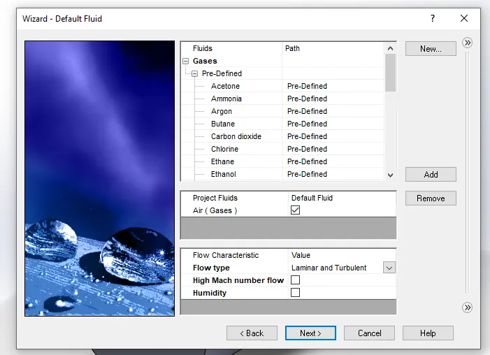
Fluid Type
Thermodynamic Parameters
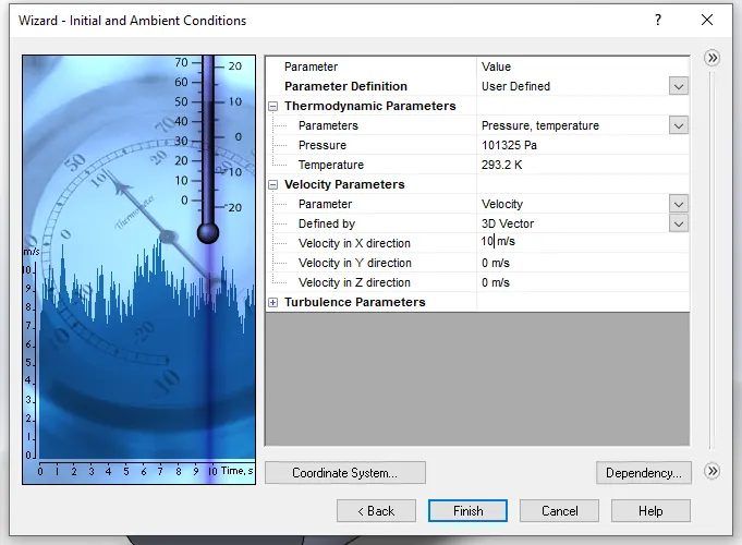
Velocity is 10 m/s along X direction as per the baseline velocity.
It can be changed as per the imput data give.
2.Then to create Cut Plot in the Middle of the Cylinder
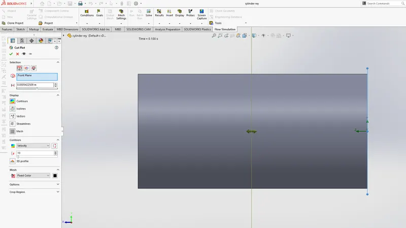
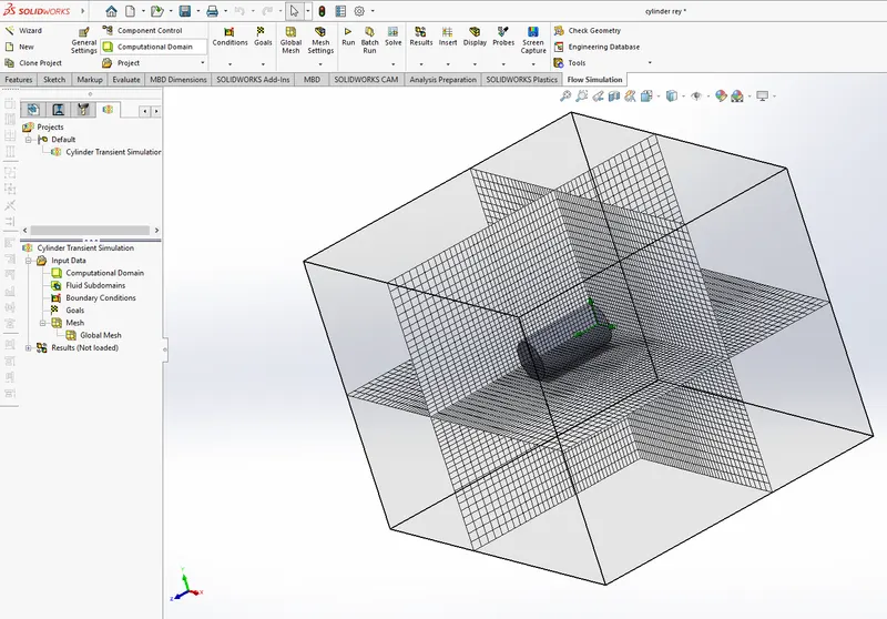
Set the Global Mesh Variable to 5
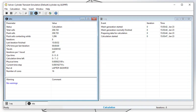
3.After that Click on Run and let the Solver Finish Calculations
4.Once the calculations are done look into the Results.
RESULTS
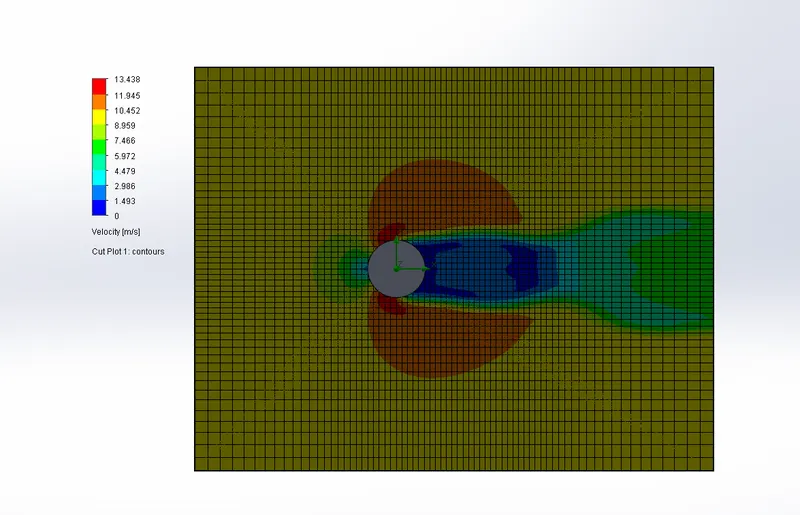
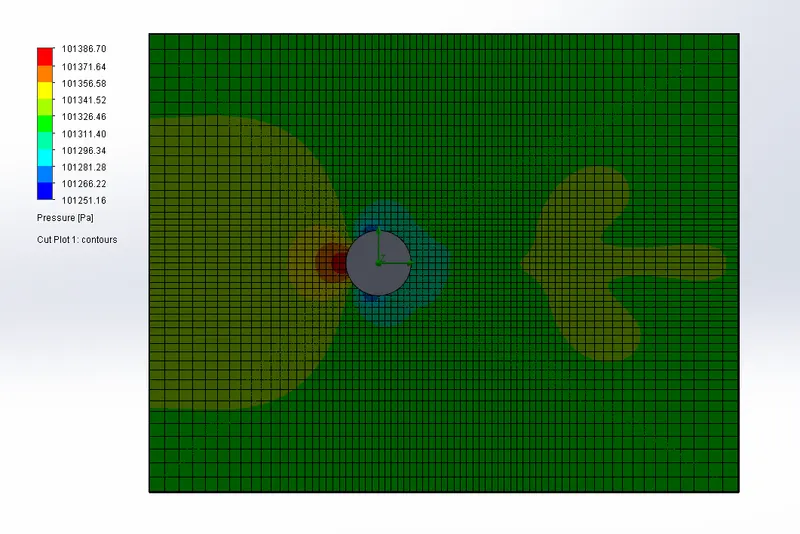
For Baseline Condition
1.Velocity Plot
2. Pressure Plot
BaseLine Animations
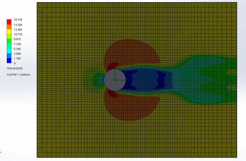
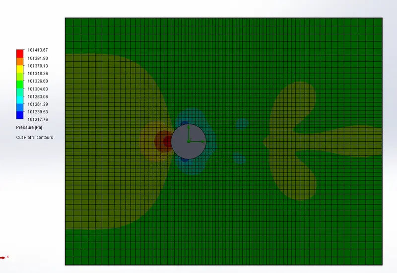
For Re increased by 20%
1.Velocity plot
2. Pressure Plot
Animations
For Re increased by 40%
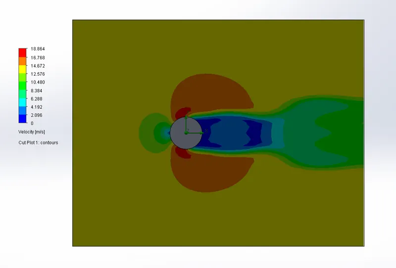
1.Velocity Plot
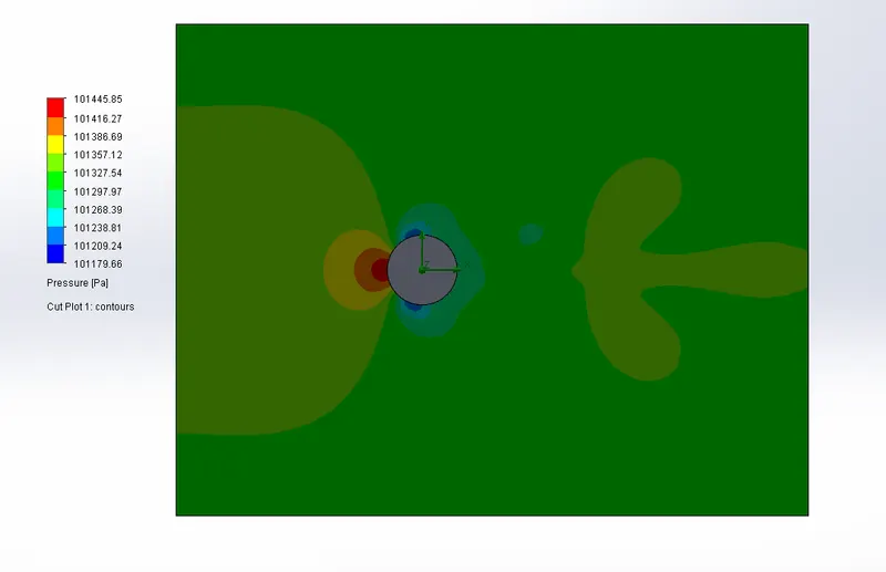
2. Pressure Plot
Animations
For Re increased by 100%
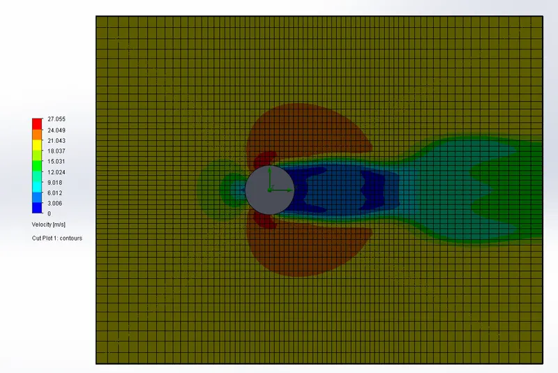
1.Velocity Plot
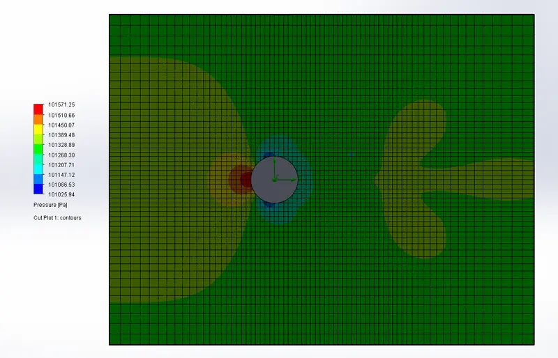
2.Pressure Plot
Animations
OBSERVATIONS AND CONCLUSION:
- We can clearly see from the following simulations that as the velocity increases , the reynolds number also increases ,hence changing the flow from laminar to turbulent.
- There is also pressure difference between the front and back of the cylinder.
- The flow becomes more convergent over the output side.
- High pressure is generated near the inlet side of the cylinder.
- Vortex formation takes place at the side of the cylinder which is opposite to velocity flow.
- The variation is mainly seen at the right side of the cylinder.