Final Project: Electric Rickshaw modelling

AIM:

• To create a matlab Simulink model of an E-rickshaw(three wheeler) and analyse its performance.
• modelling, design and power management of a energy storage system for a three-wheeled light electric vehicle under various driving conditions

OBJECTIVES:

• Select a suitable configuration of an electric model
• Selecting various specifications for every component
• Modelling the vehicle simulating it under varying parameters and observe its performance
• Compare and analyse the results for different driving conditions and parameters.
• To change motor specifications and observe variation in output results

ABSTRACT:

Global efforts towards minimizing greenhouse gas emissions are required to reduce the environmental issues caused by conventional combustion engine vehicles. Alternate clean and green modes of transportation such as electric vehicles are required in place of conventional vehicles. As a cheaper version of electric vehicle, electric rickshaws (popularly known as E-rickshaws or tuk-tuks) are most popular in India. This work deals with the modelling of popular e-rickshaws in MATLAB/Simulink. Software simulations are much helpful for quickly analysing the distinct features of the electric vehicle, such as aerodynamic design, battery energy density, motor output, curb weight, etc and to visualize the effects on its performance due to variation in various parameters and environmental conditions. Therefore, simulations were performed with Simulink model of conceptual e-rickshaw model with heterogeneous battery pack.

INTRODUCTION

Electric vehicles are now in revolutionary phase in India, but not so significantly in cars [1-2]. There are approximately 1.5 million electric rickshaws in India in comparison to 1.35 million electric rickshaws in China. Electric rickshaws (popularly known as e-rickshaws or tuk-tuks) are popular in several cities of India since 2008 as a result of their low fuel cost, and less human effort compared to pedal rickshaws. They are well accepted as an alternative to combustion engine-powered rickshaws and pedal rickshaw .

The electric rickshaws are powered by brushless dc motors ranging from 850-1150 watts and mostly produced either in China or India. An electric rickshaw offers a cheaper and eco-friendly transport facility to the low-income people . An illustration of E-rickshaw specifications, investment and net-income is shown in Figure 1.

The major reasons for the rise of e-rickshaw are:

1. They require lower investment than an Auto-Rickshaw and quite pleasing daily earnings than cycle rickshaws.
2. They have lower running cost as E-Rickshaw charging is easily available with conventional single phase socket at home and low operating cost model for rickshaw owners.
3. E-Rickshaw is one of the best options for passengers for quick, safe and cost effective last mile connectivity.
4. They provide mass scale employment and good source of income to the traditional rickshaw puller

Methodology

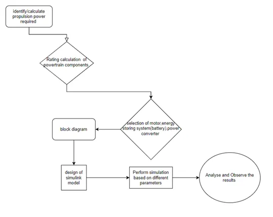
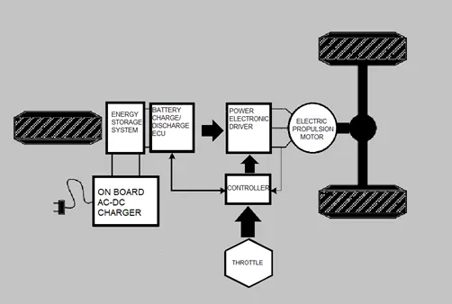
Figure 2: An Illustration of drivetrain of an E-rickshaw

PROCEDURE:

With necessary assumptions, calculate the force and power required to push / pull the vehicle.

Various forces acting on the vehicle,

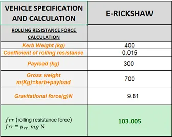
1. Rolling resistance
2. Aerodynamic force

• Hill climbing

And hence we calculate the total tractive power required for propulsion

ASSUMPTIONS AND PARAMETERS:

• A brushed permanent magnet dc motor with a li-ion battery of suitable rating has to be used
• The motor and controller efficiency is also assumed
• Motor losses and thermal losses also have been assumed
• The calculation is for reference purpose

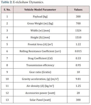
TRACTIVE POWER CALCULATION

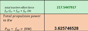
HENCE THE MOTOR MUST PROVIDE THE REQUIRED PROPULSION POWER UTILISING THE ENERGY FROM THE LI-ION BATTERY TO MOVE THE VEHICLE FORWARD

SIMULINK MODELLING

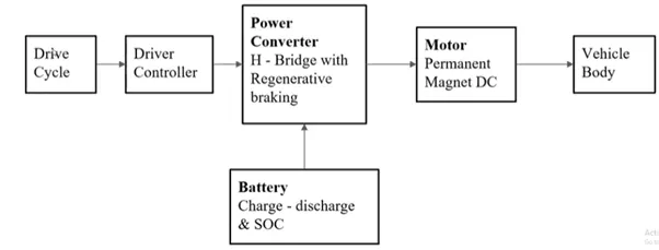
In the designed Electric Rickshaw main blocks are Battery, drive cycle, controller, DC Motor, Vehicle body & Transmission system. Drive cycle is the input data like how a human drive his actual vehicle here FTP75, WOT & Excel (Manually Prepared in Excel sheet) drive cycles are used to make the designed vehicle to give the output how it reacts to the drive cycle. The main objective is to obtain the speed by the driver, to estimate the temperature of Motor and Controller, to estimate the sates of charge (SOC), distance travelled by the vehicle. There is a SOC block that will estimate the state of charge of a battery, distance is calculated by speed and time parameters for all the three Drive cycles.

SIMULINK MODEL

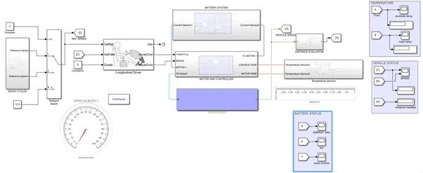
Initially the current flows to DC Motor from the battery through the DC-DC power converter to drive the motor. The required voltage will be controlled in the controller. The Controller will follow the given drive cycle reference and run the motor in the required rpm. Then the motor power is transmitted to the wheels of a vehicle through the gear box, and the controller will take the vehicle speed and compare and controlled.

SYSTEM LEVEL CONFIGURATION

1. VEHICLE DYNAMICS
2. 

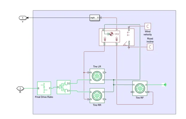
The vehicle dynamics Mainly represents the vehicle body and its physical environment. It consists various blocks mainly the tires with axle, gear transmission and vehicle chassis.

Tire(magic formula)

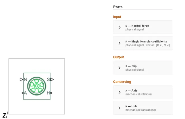
The Tire (Magic Formula) block models a tire with longitudinal behavior given by the Magic Formula [1], an empirical equation based on four fitting coefficients. The block can model tire dynamics under constant or variable pavement conditions.

The longitudinal direction of the tire is the same as its direction of motion as it rolls on pavement. This block is a structural component based on the Tire-Road Interaction (Magic Formula) block.

To increase the fidelity of the tire model, you can specify properties such as tire compliance, inertia, and rolling resistance. However, these properties increase the complexity of the tire model and can slow down simulation. Consider ignoring tire compliance and inertia if simulating the model in real time or if preparing the model for hardware-in-the-loop (HIL) simulation.

Vehicle body

https://www.mathworks.com/help/releases/R2020a/physmod/sdl/ref/vehiclebody.html

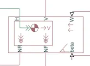
The Vehicle Body block represents a two-axle vehicle body in longitudinal motion. The vehicle can have the same or a different number of wheels on each axle. For example, two wheels on the front axle and one wheel on the rear axle. The vehicle wheels are assumed identical in size. The vehicle can also have a center of gravity (CG) that is at or below the plane of travel.

The block accounts for body mass, aerodynamic drag, road incline, and weight distribution between axles due to acceleration and road profile. Optionally include pitch and suspension dynamics. The vehicle does not move vertically relative to the ground.

The block has an option to include an externally-defined mass and an externally-defined inertia. The mass, inertia, and center of gravity of the vehicle body can vary over the course of simulation in response to system changes.

Simple Gear

https://www.mathworks.com/help/releases/R2020a/physmod/sdl/ref/simplegear.html

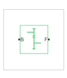
The Simple Gear block represents a gearbox that constrains the connected driveline axes of the base gear, B, and the follower gear, F, to corotate with a fixed ratio that you specify. You choose whether the follower axis rotates in the same or opposite direction as the base axis. If they rotate in the same direction, the angular velocity of the follower, ω_F, and the angular velocity of the base, ω_B, have the same sign. If they rotate in opposite directions, ω_F and ω_B have opposite signs.

2. DC PROPULSION MOTOR WITH CONTROLLER

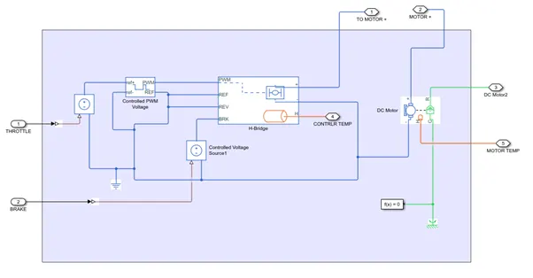
DC motor

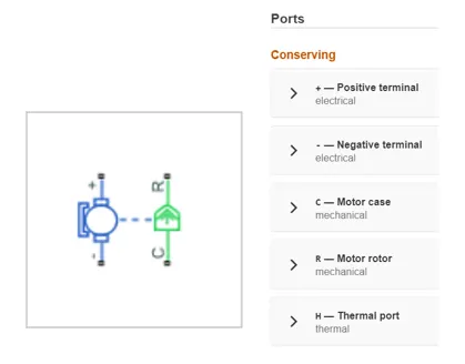
This block represents the electrical and torque characteristics of a DC motor.

The block assumes that no electromagnetic energy is lost, and hence the back-emf and torque constants have the same numerical value when in SI units. Motor parameters can either be specified directly, or derived from no-load speed and stall torque. If no information is available on armature inductance, this parameter can be set to some small non-zero value.

When a positive current flows from the electrical + to - ports, a positive torque acts from the mechanical C to R ports. Motor torque direction can be changed by altering the sign of the back-emf or torque constants.

https://www.mathworks.com/help/releases/R2020a/physmod/sps/ref/dcmotor.html#brebfy9-7

H-bridge motor driver

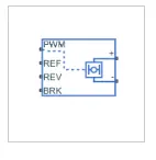
This block represents an H-bridge motor drive. The block can be driven by the Controlled PWM Voltage block in PWM or Averaged mode. In PWM mode, the motor is powered if the PWM port voltage is above the Enable threshold voltage. In Averaged mode, the PWM port voltage divided by the PWM signal amplitude parameter defines the ratio of the on-time to the PWM period. Using this ratio and assumptions about the load, the block applies an average voltage to the load that achieves the correct average load current. The Simulation mode parameter value must be the same for the Controlled PWM Voltage and H-Bridge blocks.

If the REV port voltage is greater than the Reverse threshold voltage, then the output voltage polarity is reversed. If the BRK port voltage is greater than the Braking threshold voltage, then the output terminals are short circuited via one bridge arm in series with the parallel combination of a second bridge arm and a freewheeling diode. Voltages at ports PWM, REV and BRK are defined relative to the REF port.

https://www.mathworks.com/help/releases/R2020a/physmod/sps/ref/hbridge.html

Controlled PWM Voltage

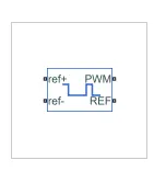
https://www.mathworks.com/help/releases/R2020a/physmod/sps/ref/controlledpwmvoltage.html.

This block creates a Pulse-Width Modulated (PWM) voltage across the PWM and REF ports. The output voltage is zero when the pulse is low, and is equal to the Output voltage amplitude parameter when high. Duty cycle is set by the input value. Right-click the block and select Simscape-> Block choices to switch between electrical +ref/-ref ports and PS input u to specify the input value.

At time zero, the pulse is initialized as high unless the duty cycle is set to zero or the Pulse delay time is greater than zero.

3. BATTERY PACK

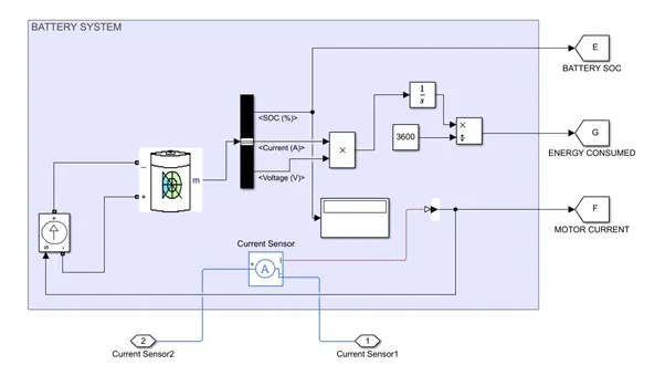
Battery

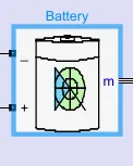
https://www.mathworks.com/help/releases/R2020a/physmod/sps/ref/battery.html

This block models a battery. If you select Infinite for the Battery charge capacity parameter, the block models the battery as a series internal resistance and a constant voltage source. If you select Finite for the Battery charge capacity parameter, the block models the battery as a series internal resistance plus a charge-dependent voltage source defined by:

V = Vnom*SOC/(1-beta*(1-SOC))

where SOC is the state of charge and Vnom is the nominal voltage. Coefficient beta is calculated to satisfy a user-defined data point [AH1,V1].

4. DRIVER INPUT WITH DRIVER CONTROLLER

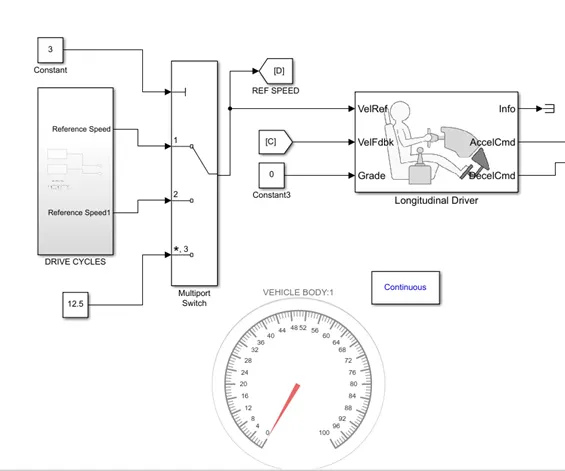
PID controller

The PID Controller block implements a PID controller (PID, PI, PD, P only, or I only). The block is identical to the Discrete PID Controller block with the Time domain parameter set to Continuous-time.

The block output is a weighted sum of the input signal, the integral of the input signal, and the derivative of the input signal. The weights are the proportional, integral, and derivative gain parameters. A first-order pole filters the derivative action.

The block supports several controller types and structures. Configurable options in the block include:

• Controller type (PID, PI, PD, P only, or I only) — See the Controller
• Controller form (Parallel or Ideal) — See the Form
• Time domain (continuous or discrete) — See the Time domain
• Initial conditions and reset trigger — See the Sourceand External reset
• Output saturation limits and built-in anti-windup mechanism — See the Limit output
• Signal tracking for bumpless control transfer and multiloop control — See the Enable tracking mode

Drive cycle

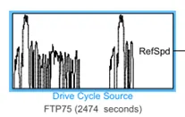
https://www.mathworks.com/help/releases/R2020a/autoblks/ref/drivecyclesource.html

The Drive Cycle Source block generates a standard or user-specified longitudinal drive cycle. The block output is the specified vehicle longitudinal speed, which you can use to:

Predict the engine torque and fuel consumption that a vehicle requires to achieve desired speed and acceleration for a given gear shift reference.

Produce realistic velocity and shift references for closed loop acceleration and braking commands for vehicle control and plant models.

Study, tune, and optimize vehicle control, system performance, and system robustness over multiple drive cycles.

Identify the faults within tolerances specified by standardized tests, including:

EPA dynamometer driving schedules1

Worldwide Harmonised Light Vehicle Test Procedure (WLTP) laboratory tests

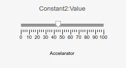
Accelarator

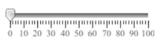
The Slider block tunes the value of the connected block parameter during simulation. For example, you can connect the Slider block to a Gain block in your model and adjust its value during simulation. You can modify the range of the Slider block's scale to fit your data. Use the Slider block with other Dashboard blocks to create an interactive dashboard to control your model.

Temperature sensors

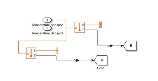
The Temperature Sensor block represents an ideal temperature sensor, that is, a device that determines the temperature differential measured between two points without drawing any heat.

Connections A and B are thermal conserving ports that connect to the two points where temperature is being monitored. Port T is a physical signal port that outputs the temperature differential value.

The block positive direction is from port A to port B. The measured temperature is determined as T = T_A – T_B.

The block has the following ports:

A

Thermal conserving port associated with the sensor positive probe.

B

Thermal conserving port associated with the sensor negative probe.

T

Physical signal output port for temperature.

RESULTS:

FOR FTP72 DRIVE CYCLE

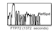
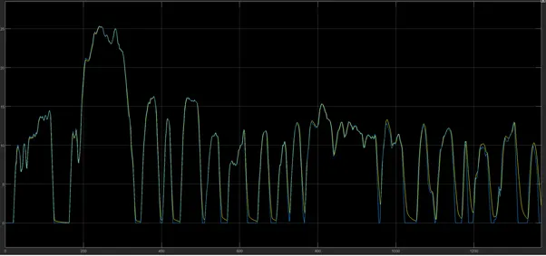
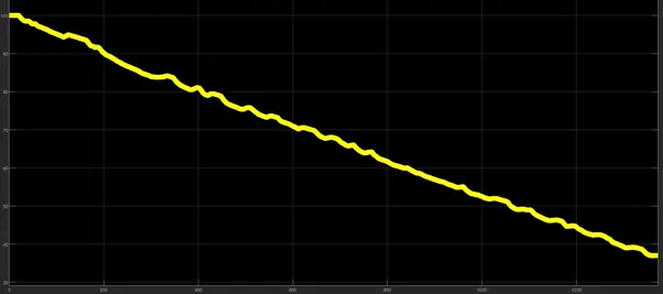
Running the vehicle with FTP72 for 1372 seconds

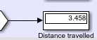
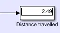
Distance covered in miles

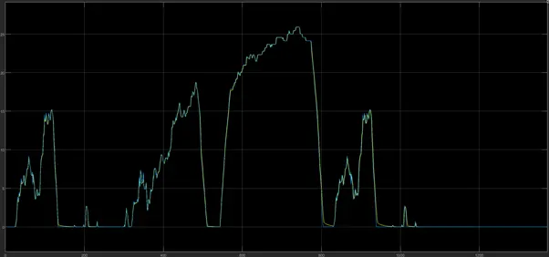
1. Vehicle speed tracking 95% to the reference speed

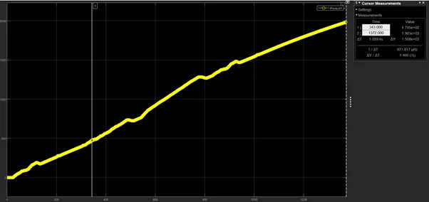
2. Total Energy consumed in kWh over the run 2.1 kWh

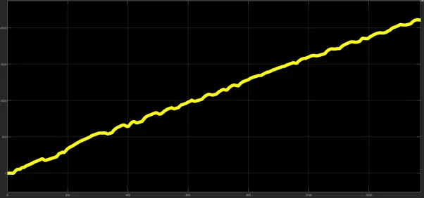
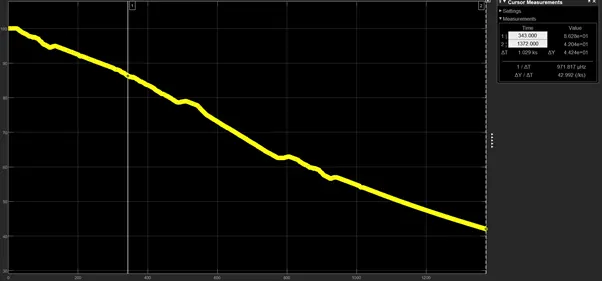
3.State of charge of battery at the end of the run= 37%

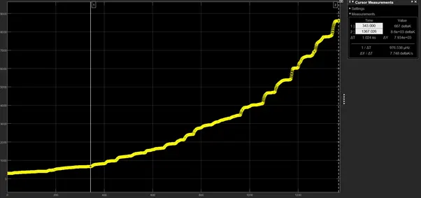
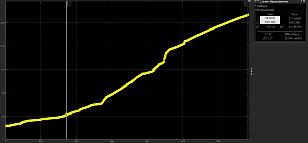
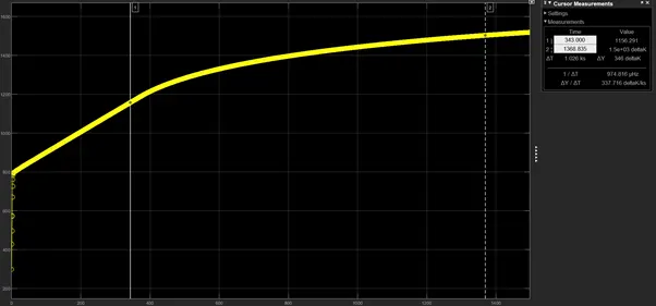
4.Motor temperature at end of the run Tm= 8600K

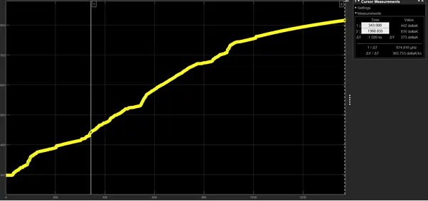
5.Controller temperature at end of run Tc=1078K

FOR HUDDS

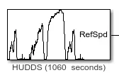
Running the vehicle with FTP72 for 1060 seconds

Distance covered in miles

1. Vehicle speed tracking 95% to the reference speed

2. Total Energy consumed in kWh over the run 1.9 kWh

3. State of charge of battery at the end of the run= 42%

4. Motor temperature at end of the run Tm= 2672K

5. controller temperature at end of the run Tc= 816K

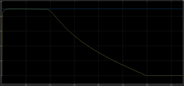
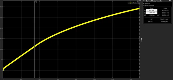
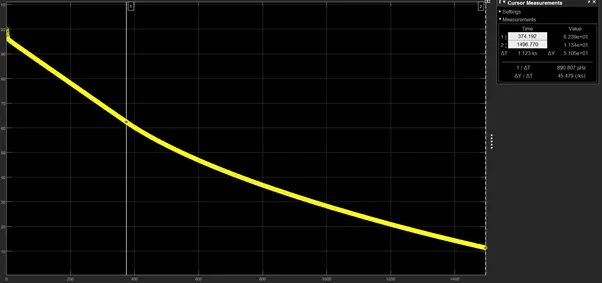
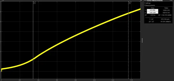
FOR CONSTANT DRIVING AT 45KMPH TILL BATTERY DRAINS

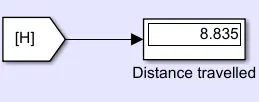
Distance covered 8.8 miles in time 1623 seconds

1. Vehicle speed tracking to the reference speed

2. Total Energy consumed in kWh over the run 2.9 kWh

3. State of charge of battery at the end of the run= 11.3%

4.Motor temperature at end of the run

5. controller temperature at end of the run

CONCLUSION

We Created a MATLAB model of electric RICKSHAW which uses lithium ion battery with suitable motor, by using suitable blocks from Simscape or Powertrain block set and we Implement the vehicle speed control using controller and generate brake and accelerator commands, we have seen System level configurations, Model parameters, the model run as per our reference input.

• In the real time application, the motor, battery & controller temperature is controlled by air cooling. Hence, the temperature of this components is not increased to this extent.
• Determined the variations of Temperature of Motor and controller, SoC% and Energy consumed by the by vehicle for all the three drive cycles

REFERENCES

file:///C:/Users/mkaif/Downloads/Simulation_and_Analysis_of_Hybrid_Solar_E-Rickshaw.pdf

https://journals.sagepub.com/doi/pdf/10.1177/0020294019858212