Final Project: Electric Rickshaw modelling

Create a detailed MATLAB model of an electric rickshaw (three wheel passenger vehicle) as per details below:

Rear wheels driven by PM brushed type motor

Assume efficiency points of motor controller and motor

Make an excel sheet of all input and assumed data

Results: For any three standard driving cycles show energy consumption, temperature rise of motor and controller for 100 km constant speed driving at 45 kmph.

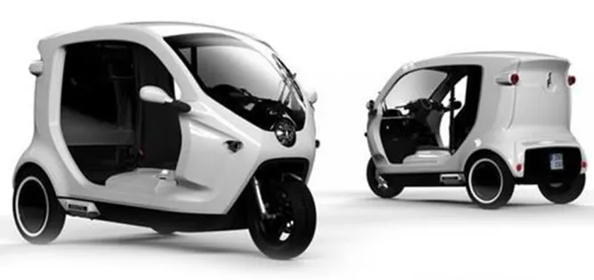
Today, the rickshaw represents over a century of rich Indian culture. Originally brought to the country from China, the rickshaw was a hand-pulled vehicle used by traders for transportation of goods. In 1914, the traders asked the governing body for permission to allow the transportation of people as passengers. The request was granted, and rickshaws became a mode of transport for the elite, although now it is used by people of all classes. Since its introduction in 1880, the rickshaw has advanced and evolved into different categories of vehicle: Hand-pulled, cycled, and motorised. Cycle rickshaws began to appear in India around 1930.

The general parameters of an ordinary auto-Rikshaw is been considered. The similar power requirement is been considered for the design of an electric Rikshaw in this simulation.

The Bajaj Auto rikshaw has the following parameters:-

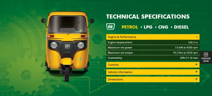
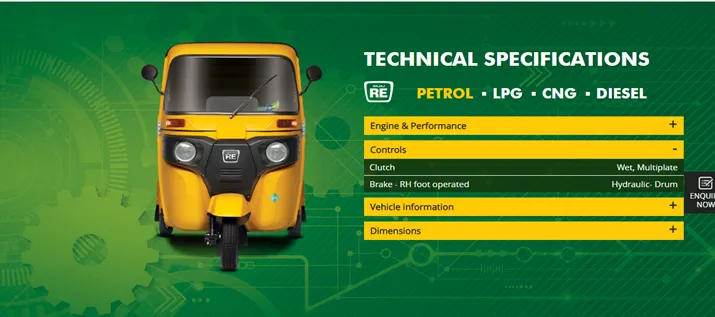
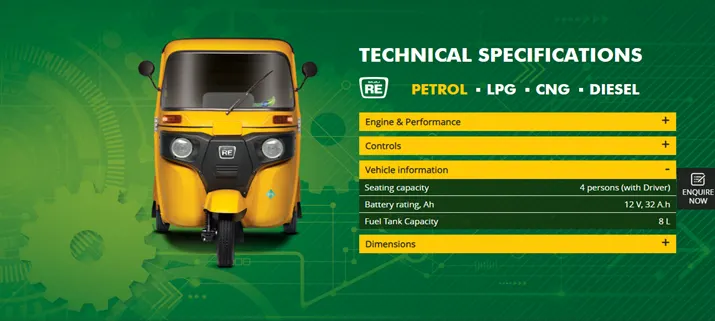
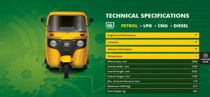
As per the above data of this Bajaj auto-rikshaw is taken as reference for the electric auto-rikshaw.

The specification considered for the electric Rikshaw are as follows:-

PM Brushed motor= 120KW , 300V

Total weight= 800kg

Overall length = 2635mm

Overall width = 1300mm

Overall height = 1692mm

Tyre size = 90x90x12, 3.2x12

Frontal area considered = 2m^2

The Simulink model for the electric Auto-rikshaw is as follows:-

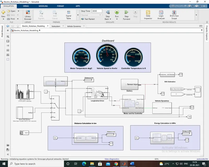
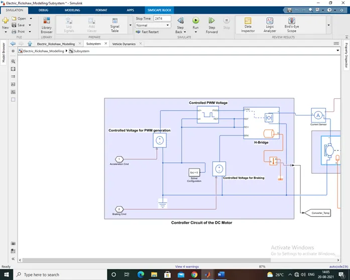
As we can see in the above model that 3 different driving cycles are been attached to the model for simulating in different driving cycle and along with it a signal builder block is been used where it provides the reference signals to the longitudinal driver block which acts as the controller, this signals are then been sent to the PID for fine tuning of the signals so that the response will get better and stable this signals are then been sent through the controlled current and voltage block to the PWM and H-bridge blocks .

A battery subsystem is been constructed by lithium ion cell. The motor is connected to the differential of the rikshaw at the rear wheel and in this way the model is constructed out.

Vehicle Subsystem :-

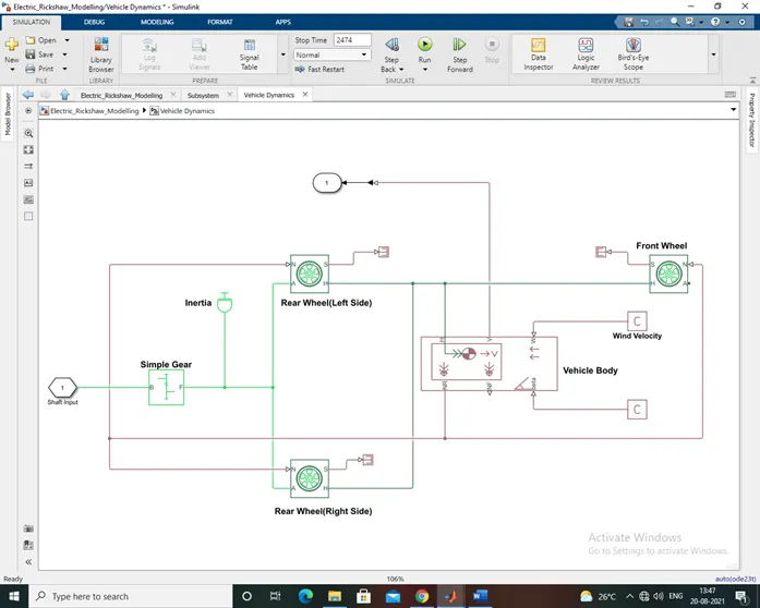
The MATLAB model is been created for the simulation of an electric vehicle , by assuming certain parameters and conditions while designing the model.

While developing this simulation the first of all frame of the vehicle is been modelled assuming the general parameters such as weight of the vehicle , frontal area , aerodynamic drag , rolling resistance for tires , air density etc. for this the VEHICLE BODY block is been used ,the graphical representation of block is as shown below-

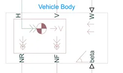
Connection H is the mechanical translational conserving port associated with the horizontal motion of the vehicle body.

Connections V, NF, and NR are physical signal output ports for vehicle velocity and front and rear normal wheel forces, respectively.

Connections W and beta are physical signal input ports corresponding to headwind speed and road inclination angle, respectively.

The mass of the vehicle = 800 kg

No. of wheel axle per =2

Horizontal distance from CG to front axle= 1.4m

Horizontal distance from CG to rear axle= 1.6m

CG height above ground= 0.5m

Gravitational acceleration= 9.81 m/s

Drag:-

Frontal area:2 m^2

Drag coefficient:0.4

Air density:1.18 kg/m^3

The parameters for vehicle body block are as follows-

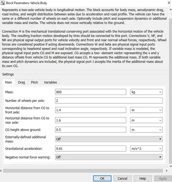
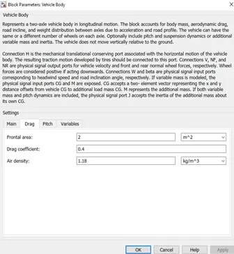
The 3 tyres are been connected to the chassis , for this the Tire (magic formula) block is been used.

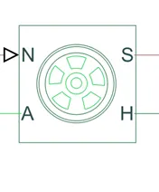
The block looks as shown above it consists of 4 ports:-

Connection A is the mechanical rotational conserving port for the wheel axle.

Connection H is the mechanical translational conserving port for the wheel hub through which the thrust developed by the tire is applied to the vehicle.

Connection N is a physical signal input port that applies the normal force acting on the tire. The force is considered positive if it acts downwards.

Connection S is a physical signal output port that reports the tire slip.

In this way 3 tire are been used one for the front wheel and two for the back wheel.

The parameters of the block are as follows:-

Rated vertical load: 4000N

Peak longitudinal force at rated load: 3500N

Slip at peak force at rated load (percent): 10

Geometry :-

Rolling radius: 0.32m

Dynamics:-

Compliance: No compliance - Suitable for HIL simulation

Inertia: No inertia

Advanced :-

Velocity threshold:0.1 m/s

Simple gear box:-

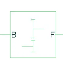
Connections B (base) and F (follower) are mechanical rotational conserving ports.

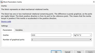
Inertia block:-

Block parameters :-

For calculation of the velocity , we have created , the block basically consists of PS-simulink converter , gain and zero order hold.

Gain block :- 1.61

Zero order hold :- 0.01

Battery Subsystem :-

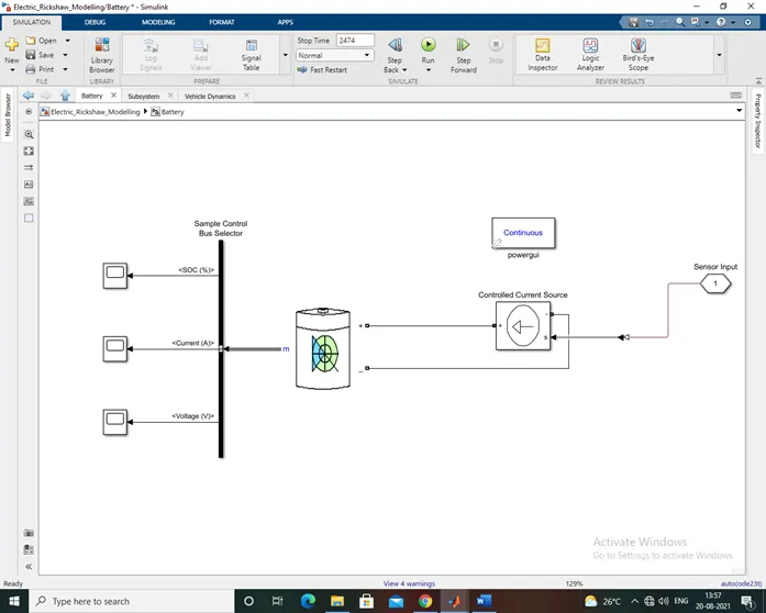
Battery Configuration :-

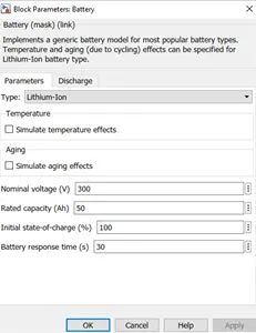
The lithium ion battery pack is been selected.

Parameters:-

Nominal voltage(V)- 300

Rated capacity (Ah)- 50

Initial state of charge(%)-100

Battery response time(s)- 30

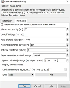
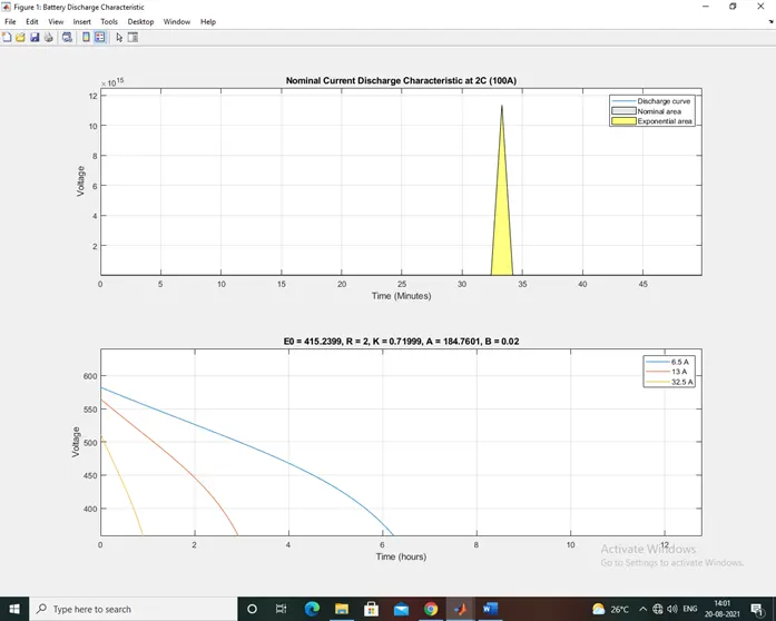
Discharge:-

Max capacity(Ah)-50

Cut off voltage (V)-300

Fully charged voltage(V)-400

Nominal discharge current(A)-100

Internal resistance (Ohms)-2

Capacity (Ah) at nominal voltage-4.8835

Exponential zone [Voltage (V), Capacity (Ah)]- [330 150]

Discharge current [i1, i2, i3,...] (A)- [6.5 13 32.5]

The discharge rate plot will be as follow-

Controlled current source :-

The controlled current source block converts the Simulink signal into equivalent current signal which is the connected to the battery . the AC or DC supply can be selected in the block.

The current direction is been showed by the direction of arrow. The positive terminal of controlled current source is connected to the negative of the battery and negative is connected to the positive of the battery.

Battery :-

The battery parameters are set as mention above.

Bus selector block :-

The bus selector allows us to take the output from the battery to check the parameters of the battery like current , voltage , SOC , etc.

PowerGui block :-

PowerGui block allows us to select between different method to solve the model.

SOC subsystem :-

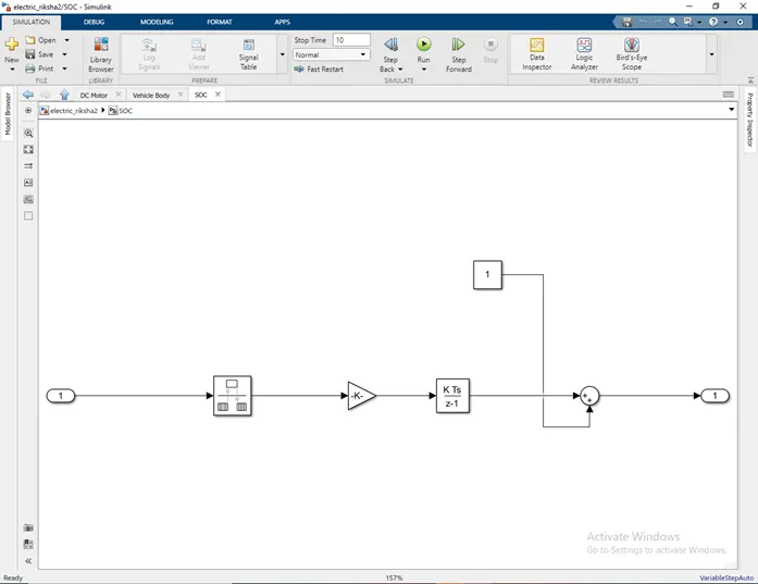
The soc subsystem consists of following blocks :-

• Rate transition
• Gain
• Discrete time integration

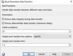
Rate transition Block :-

This block is used to transmit data from output of one block operating at one rate to the input of other block operating at different rate.

Gain Block :-

The gain block multiples the input to a certain fixed level.

Here the gain given is = 1/(75/3600) , here 75 is the battery ampere and 3600 is the seconds.

Discrete Time Integration:-

The Discrete Time Integration block is used for:-

• Define initial conditions on the block dialog box or as input to the block
• Define an input gain (K) value
• Output the block state
• Define upper and lower limits on the integral
• Reset the state with an additional reset input

Sum block :-

In this negative terminal of sum block will be connected to Discrete Time Integration and positive to the constant block.

H-Bridge , PWM and Longitudinal Driver Block &DC Motor

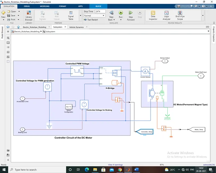
The DC motor with temperature sensor is as follows:-

The subsystem consists of following blocks:-

• DC Motor
• Ideal Rotational Motion sensor
• PS-Simulink converter

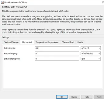
The parameters of DC Motor block are as follows:-

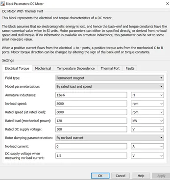
Parameters :-

Field type: Permanent magnet

Model parameterization: By rated load and speed

No-load speed: 8000 rpm

Armature inductance: 12e-6 H

Rated speed (at rated load): 6000 rpm

Rated load (mechanical power): 120kw

Rated DC supply voltage: 300 V

Rotor damping parameterization: By no load current

Mechanical Parameters :-

Rotor inertia: 0.01 g*cm^2

Rotor damping: 0 N*m/(rad/s)

Initial rotor speed: 0 rpm

Temperature dependence :-

Resistance temperature coefficient: 93e-3 1/K

Measurement temperature: 25 degC

Ideal rotational motion sensor:-

This block measures angular velocity or angle in a mechanical rotational network. The sensor is ideal since it does not account for inertia, friction, delays, energy consumption, and so on.

The connection of PWM and H-Bridge are as follows:-

Parameters of PWM block:-

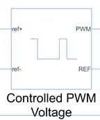
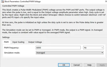
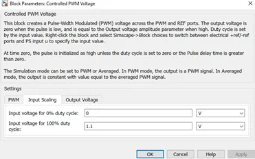
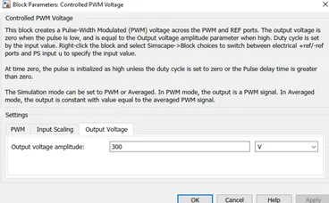
This block creates a Pulse-Width Modulated (PWM) voltage across the PWM and REF ports. The output voltage is zero when the pulse is low, and is equal to the Output voltage amplitude parameter when high. Duty cycle is set by the input value. Right-click the block and select Simscape->Block choices to switch between electrical +ref/-ref ports and PS input u to specify the input value.

At time zero, the pulse is initialized as high unless the duty cycle is set to zero or the Pulse delay time is greater than zero.

The Simulation mode can be set to PWM or Averaged. In PWM mode, the output is a PWM signal. In Averaged mode, the output is constant with value equal to the averaged PWM signal.

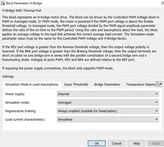
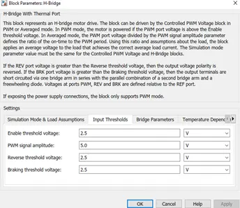
H-Bridge parameters :-

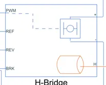
This block represents an H-bridge motor drive. The block can be driven by the Controlled PWM Voltage block in PWM or Averaged mode. In PWM mode, the motor is powered if the PWM port voltage is above the Enable threshold voltage. In Averaged mode, the PWM port voltage divided by the PWM signal amplitude parameter defines the ratio of the on-time to the PWM period.

Bridge parameters :-

Output voltage amplitude: 300 v

Total bridge on resistance:0.1 ohm

Freewheeling diode on resistance: 0.05 ohm

Measurement temperature: 298.15k

Temperature dependence:-

Total bridge on resistance at second measurement temperature: 0.1 ohm

Freewheeling diode on resistance at second measurement temperature: 0.05 ohm

Second measurement temperature: 398.15 k

Thermal Port :-

Thermal mass: 100 J/k

Initial temperature: 298.15 k

Controlled Voltage Source :-

The block represents an ideal voltage source that is powerful enough to maintain the specified voltage at its output regardless of the current passing through it.

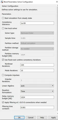
Solver configuration :-

Defines solver settings to use for simulation.

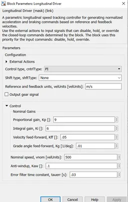
Longitudinal Driver Block:-

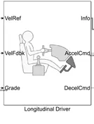
A parametric longitudinal speed tracking controller for generating normalized acceleration and braking commands based on reference and feedback velocities.

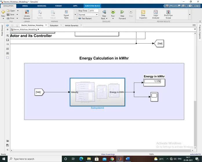
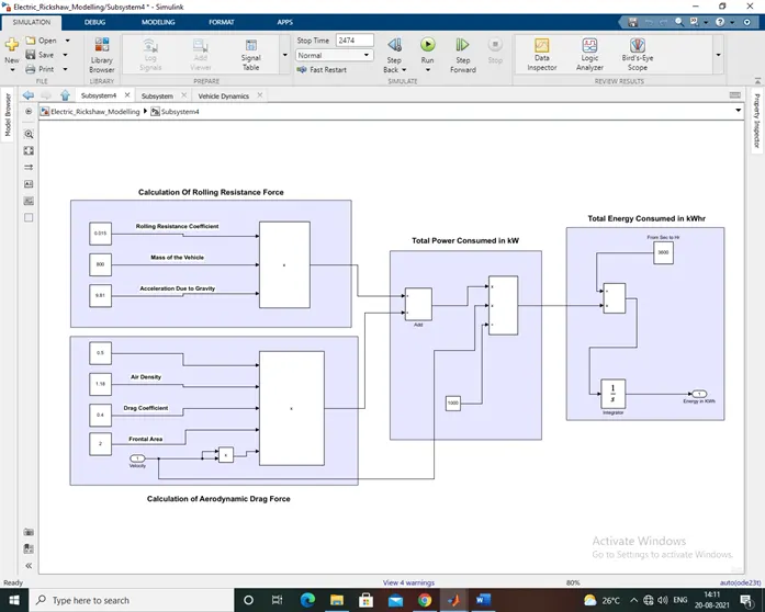
Energy Consumption calculation Subsystem :-

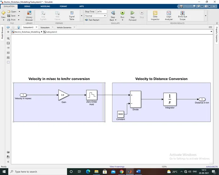
Velocity in m/sec to km/hr conversion and velocity to distance calculation:-

Results :-

The FTP75 driving cycle is been selected for the first trial

The energy consumed for FTP75 driving cycle is 1.178KWhr

Driving cycle tracing output:-

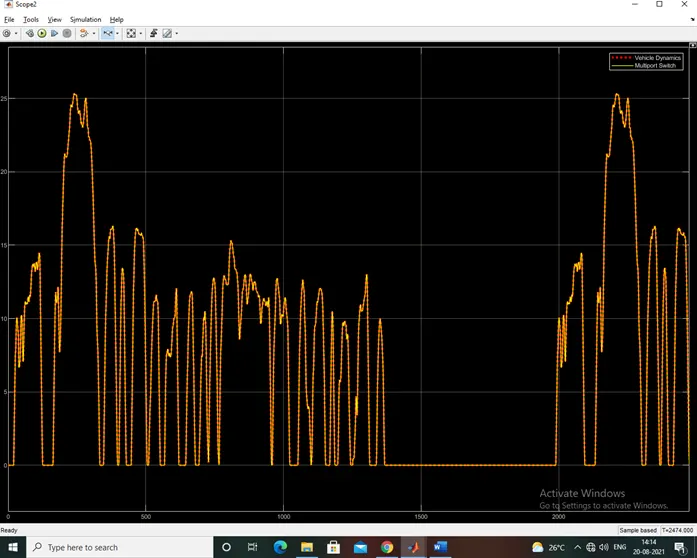
From this scope its clear that the actual speed and the reference speed is been tracked properly , the tracement is absolutely fine.

Motor temperature and controller temperature scope :-

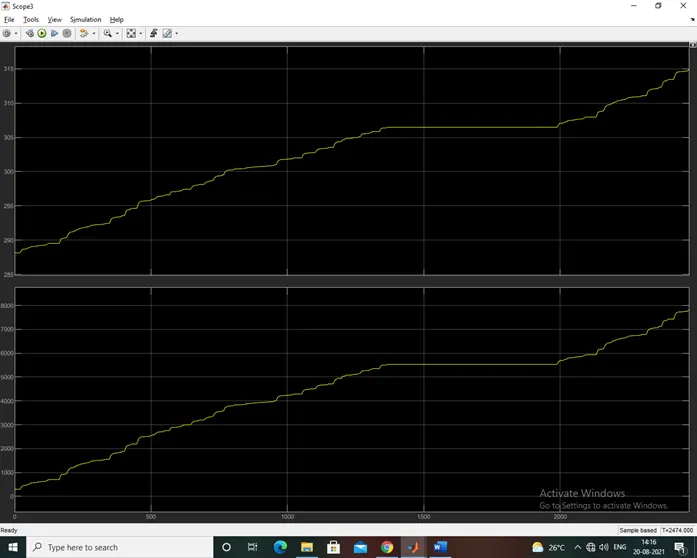
The highest temperature that the motor is going for FTP75 driving cycle is near about 315 degc

And of the controller is 7800 k.

Second run :-

The electric rikshaw is been tested for 100km at a speed of 45km/hr the results obtained after the simulation ares are as follows :-

The reference speed and the actual speed tracking scope results :-

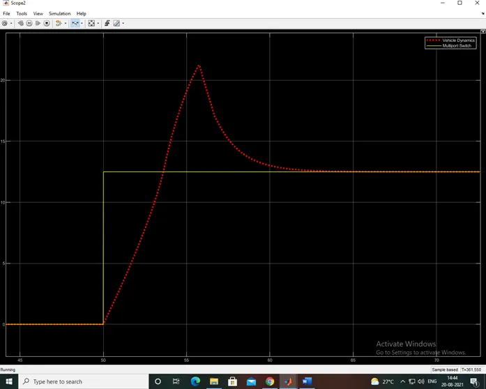
From this scope it seen that the vehicle is tracking the reference speed but at the starting of the cycle the overshoot in the speed is been observed and the speed is peaked upto 21m/s after that its able to trace the actual speed of 12.5 m/s which is equal to 45km/hr.

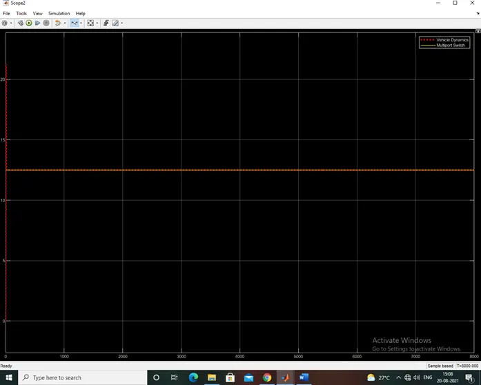
Motor and controller scope results:-

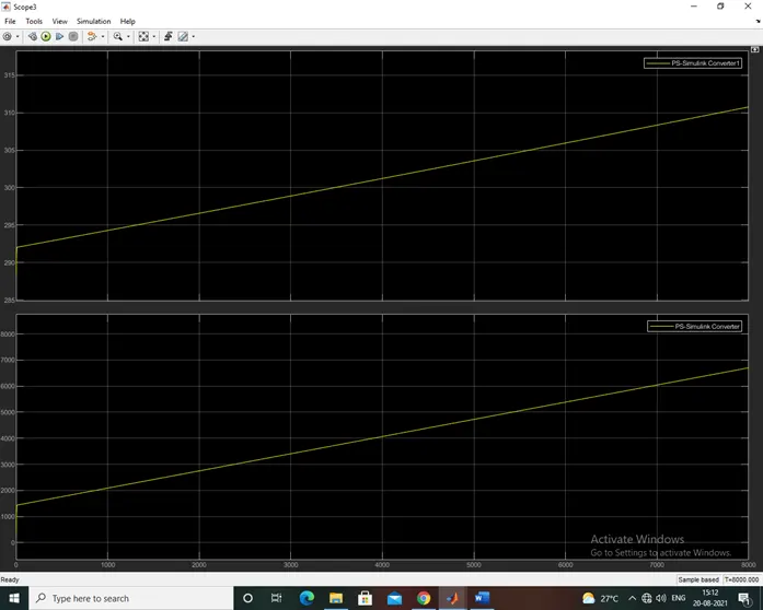
The highest temperature that the motor is going for 100km at 45km/hr speed is near about 311 degc

And of the controller is 6689 k.

Note :-I have attached the simulink model pls check it.