Final Project: Electric Rickshaw modelling

AIM:

To design a matlab model of an electric rickshaw (three wheel passenger vehicle)

OBJECTIVES:

• Rear wheels driven by PM brushed type motor
• Assume efficiency points of motor controller and motor
• Make an excel sheet of all input and assumed data

EXPLANATION AND MODELLING:

Electric Rickshaw

Electric rickshaw have been becoming more popular in some cities since 2008 as an alternative to auto rickshaws and pulled rickshaws because of their low fuel cost, and less human effort compared to pulled rickshaws. They are being widely accepted as an alternative to petrol/diesel/CNG auto rickshaws. They are three-wheelers powered by an electric motor ranging from 650 to 1400 Watts. They are mostly manufactured in India and China, only a few other countries manufacture these vehicles. Battery-run rickshaws could be a low-emitter complementary transport for the low-income people, who suffer most from a lack of transport facility, if introduced in a systematic manner according to experts.

Evolution of electric vehicles

The electric automobile did not easily develop into a viable means of transportation. Research waned from 1920 to 1960 until environmental issues of pollution and diminishing natural resources reawakened the need of a more environmentally friendly means of transportation. Technologies that support a reliable battery and the weight of the needed number of batteries elevated the price of making an electric vehicle. In 1837, Robert Davidson of Scotland appears to have been the builder of the first electric car, but it wasn't until the 1890s that electric cars were manufactured and sold in Europe and America. During the late 1890s, United States roads were populated by more electric automobiles than those with internal combustion engines.

Block diagram

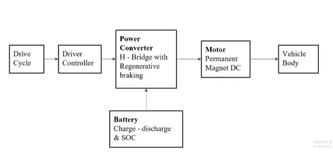
In the designed Electric Rickshaw main blocks are

• Battery
• drive cycle
• controller
• DC Motor
• Vehicle body &amp
• Transmission system.

Drive cycle is the input data like how a human drive his actual vehicle here FTP75, WOT & Excel (Manually Prepared in Excel sheet) drive cycles are used to make the designed vehicle to give the output how it reacts to the drive cycle. The main objective is to obtain the speed by the driver, to estimate the temperature of Motor and Controller, to estimate the sates of charge (SOC), distance travelled by the vehicle. There is a SOC block that will estimate the state of charge of a battery, distance is calculated by speed and time parameters for all the three Drive cycles.

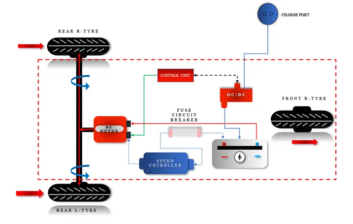
let us assume efficiency points of motor controller and motor generally in real life

The motors typically have efficiency of over 80%, and the controllers in the 95% range.

MATLAB SIMULINK MODEL

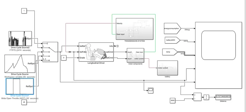
Initially the current flows to DC Motor from the battery through the DC-DC power converter to drive the motor. The required voltage will be controlled in the controller. The Controller will follow the given drive cycle reference and run the motor in the required rpm. Then the motor power is transmitted to the wheels of a vehicle through the gear box. and the controller will take the vehicle speed and compare and controlled.

MODEL PARAMETERS

DRIVE CYCLE

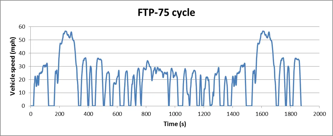
Drive cycle is assumed as the driver's input of a vehicle, it replaced how a driver will drive a vehicle. Here I have used three drive cycles which is used to test the vehicle performances. These drive cycle will have high speed, low speed, braking conditions in it. There are different drive cycles like WOT, FTP75 etc., Here in this model I have used FTP 75, WOT & Manually prepared in excel Drive Cycle source.

Generates a standard or user-specified longitudinal drive cycle. The block output is the vehicle longitudinal speed. You can import drive cycles from:

• Predefined sources
• Work space
• .mat,xlsx,slx and text files

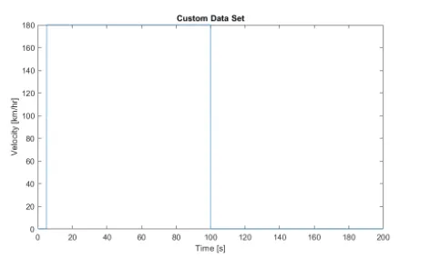
WIDE OPEN THROTTLE

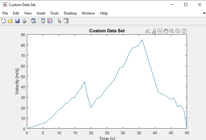
Manually prepared drive cycle

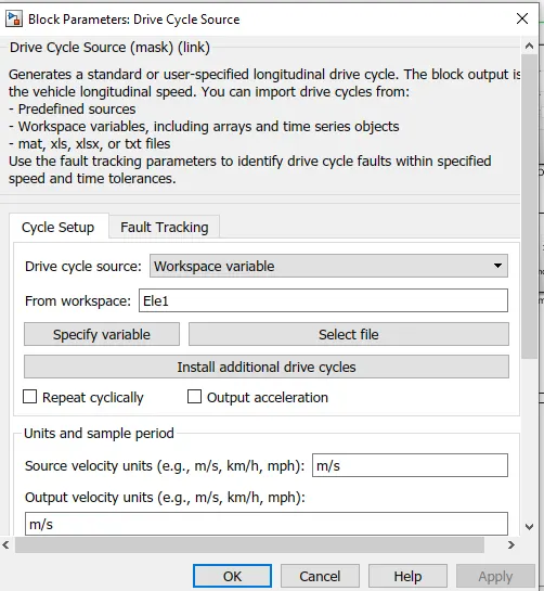
Create a drive cycle in excel then import to the work space

then double click on the drive cycle block , Drive cycle source : workspace and type the variable which is import to the work space.

All the three drive cycle are controlled through mutliport switch by providing constant to the port.

DRIVE CONTROLLER

Longitudinal drive

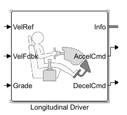
A parametric longitudinal speed tracking controller for generating normalized acceleration and braking commands based on reference and feedback velocities.

Use the external actions to input signals that can disable, hold, or override the closed-loop commands determined by the block. The block uses this priority for the input commands: disable, hold, override.

Drive cycle is connected to a longitudinal driver, it has six ports namely velocity reference, velocity feedback, grade, info, Acceleration, Deceleration.

VelRef is given by the drive cycle data and VelFdbk is given by the output of the motor. These two will get compare and the acceleration or deceleration output will be given to the motor controller. Accelcmd is given the PWM generator block and deccelcmd is given to the regenerative port of the h-bridge which uses to generate regenerative braking. Info is used to get any other data from a longitudinal driver block. The grade is to give the input of gradeability to the driver block. This block helps to generate regerate the driver's conditions of the vehicle using the driver cycle block.

Motor & controller

Motor type

DC motor ( PM brushed type motor)

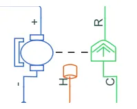
This block represents the electrical and torque characteristics of a DC motor includes Thermal port to sence the temperature of Motor.

The block assumes that no electromagnetic energy is lost, and hence the back-emf and torque constants have the same numerical value when in SI units. Motor parameters can either be specified directly, or derived from no-load speed and stall torque. If no information is available on armature inductance, this parameter can be set to some small non-zero value.

When a positive current flow from the electrical + to - ports, a positive torque acts from the mechanical C to R ports. Motor torque direction can be changed by altering the sign of the back-emf or torque constants.

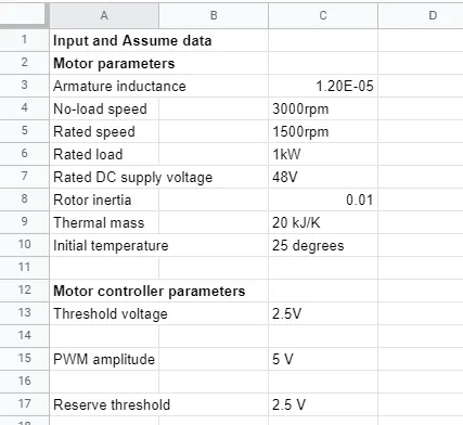
Motor parameters

• Armature inductance 12e-6
• No-load speed 3000rpm
• Rated speed 1500rpm
• Rated load 1 kW
• Rated DC supply voltage 48V
• Rotor inertia 0.01
• Thermal mass 20 kJ/K
• Initial temperature 25 degrees

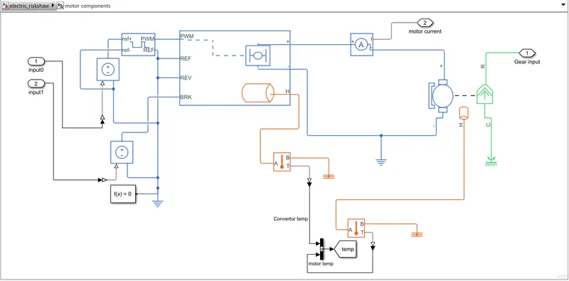
TheMotor controller will get input from the longitudinal driver. Its tasks are to control the speed of the motor and drive according to the input of the driver. Majorly motor controlled we designed had two main parts named PWM voltage generator and H-Bridge.

Input1 is getting from the accelmd of a longitudinal driver and it is given to a controlled voltage source block where it is input to the controlled PWM voltage. Controlled PWM voltage will generate a PWM signal in such a way that H-bridge will generate the required voltage to operate the DC motor for the given driver input. PWM voltage block negative reference and REF are grounded and REF of H-bridge respectively. H-bridge is a motor controller that has IGBT components aligned in the shape of H and will operate only two at a time respectively to the input of the signal from the PWM block. When deceleration occur this H-bridge will give an output from the positive and negative terminals of it. These negative & positive terminals are later connected to the DC motor and battery. All these components are the simscape electrical components so they need a connection to the solver configuration block which helps to solve the simulation.

Controlled PWM voltage source.

This block creates a Pulse-Width Modulated (PWM) voltage across the PWM and REF ports. The output voltage is zero when the pulse is low, and is equal to the Output voltage amplitude parameter when high. Duty cycle is set by the input value. Right-click the block and select Simscape->Block choices to switch between electrical +ref/-ref ports and PS input u to specify the input value.

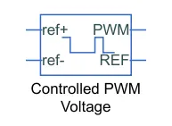
At time zero, the pulse is initialized as high unless the duty cycle is set to zero or the Pulse delay time is greater than zero.

The Simulation mode can be set to PWM or Averaged. In PWM mode, the output is a PWM signal. In Averaged mode, the output is constant with value equal to the averaged PWM signal.

Power Converter

H-bridge

It is used as a DC_DC converter

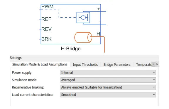
This block represents an H-bridge motor drive. The block can be driven by the Controlled PWM Voltage block in PWM or Averaged mode. In PWM mode, the motor is powered if the PWM port voltage is above the Enable threshold voltage. In Averaged mode, the PWM port voltage divided by the PWM signal amplitude parameter defines the ratio of the on-time to the PWM period. Using this ratio and assumptions about the load, the block applies an average voltage to the load that achieves the correct average load current. The Simulation mode parameter value must be the same for the Controlled PWM Voltage and H-Bridge blocks.

If the REV port voltage is greater than the Reverse threshold voltage, then the output voltage polarity is reversed. If the BRK port voltage is greater than the Braking threshold voltage, then the output terminals are short circuited via one bridge arm in series with the parallel combination of a second bridge arm and a freewheeling diode. Voltages at ports PWM, REV and BRK are defined relative to the REF port.

If exposing the power supply connections, the block only supports PWM mode.

Motor controller parameters

Threshold voltage 2.5 V

PWM amplitude 5V

Reserve threshold 2.5VB

Braking voltage 2.5 V

Output voltage 200V

Temperature sensor

The temperature sensor is used to measure the temperature in H-bridge and motor.

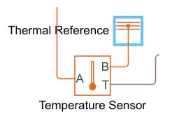
This block measures temperature in a thermal network. There is no heat flow through the sensor. The physical signal port T reports the temperature difference across the sensor. The measurement is positive when the temperature at port A is greater than the temperature at port B.

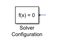
Solver configuration

Defines the solver settings to use for simulation

References

1. Electrical reference: It act as a ground . All the electrical parameters connected to it.
2. Mechanical reference: All the mechanical parameters are connected to it.
3. Thermal reference: All the thermal components are connected to it.

Battery

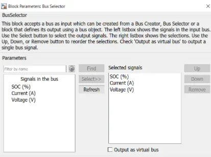
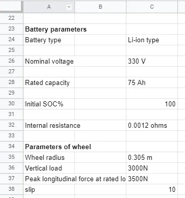
Battery parameters

Battery type Li-ion type

Nominal voltage 330V

Rated capacity 75 Ah

Initial SOC% 100

Internal resistance 0.0012 ohms

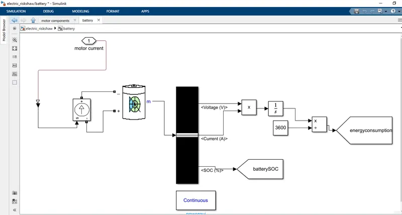
The battery is required to power the controller and motor. The controller uses the battery power according to produce the input given by the motor to obtain maximum speed. The battery is also used to power every electrical component in the vehicle. The battery has two stage one is charging and another one is discharging state. The battery is of 75Ah capacity.

The battery as a series internal resistance plus a charge-dependent voltage source defined by:

`V=(V_n.SoC)/((1-beta).(1-SoC)`

where SoC is the state of charge and Vnom is the nominal voltage. Coefficient beta is calculated to satisfy a user-defined data point [AH1,V1].

The battery has a positive and negative terminal which is given the voltage-controlled source where the battery consumption is controlled by the motor controller and then it is given to the SOC block.

State of charge

SoC is the percentage or level of battery presents after certain travel or consumption of battery charge by the vehicle. In the designed vehicle battery charge or SOC is calculated by the giving it to the rate transition and then to gain where 1/(nominal battery capacity) then to a discrete-time integrator and it will get minus from the 1 as it is considered a 100% of battery and it is multiplied with 100 to get percentage of battery.

The majority of blocks are simscape blocks where physical to simulink converter is used to convert the physical signal from simscape block to simulink signal.

Vehicle body and transmission

Motor will produce the rotational output which will give to the vehicle body and transmission system. The rotational output is taken by the gear system here to maintain the constant speed throughout the transmission without any loss in speed from the motor to tires. Below is a diagram that is how it is how it inside the vehicle body and transmission system and in the main design, it is referred just only as a transmission system.

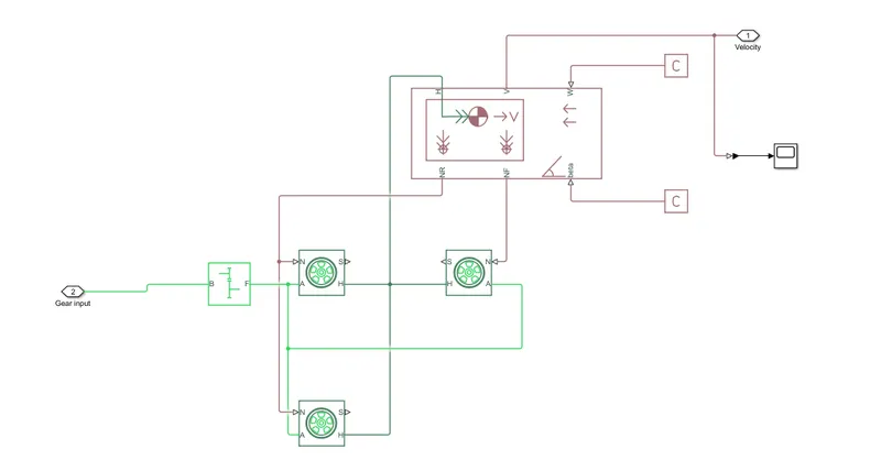
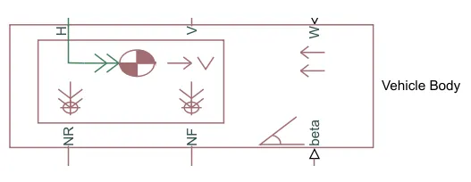
The gear output is given to axels of Rear tires, in the circuit it is shown that gear is connected to Rear wheels and front tire is free to rotational motion, thus vehicle moves forward. N is the normal force caused by the tires and it is given to the vehicle body normal force port. The vehicle body has an H-Hub, S- Tire slip, N- Normal force, A- axel connection, wind velocity, inclination angle. The tires hub is connected as a common node to the vehicle body. The vehicle body wind velocity is connected to a constant block and the beta-inclination angle is connected to another constant block where we can assign wind velocity and inclination angle as per requirement. Velocity is the output port where we can get at which speed the vehicle is moving. The velocity is taken out to the get the distance travelled and state of charge.

Vehicle body

Parameters

Mass 615kgs

No. of wheels per axle 2

Frontal area 1.48 m^2

Drag coefficient 0.5

Air density 1.18 kg/m^3

Wheels

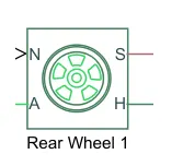
Represents the longitudinal behavior of a highway tire characterized by the tire Magic Formula. The block is built from Tire-Road Interaction (Magic Formula) and Simscape Foundation Library Wheel and Axle blocks. Optionally, the effects of tire inertia, stiffness, and damping can be included.

Connection A is the mechanical rotational conserving port for the wheel axle. Connection H is the mechanical translational conserving port for the wheel hub through which the thrust developed by the tire is applied to the vehicle. Connection N is a physical signal input port that applies the normal force acting on the tire. The force is considered positive if it acts downwards. Connection S is a physical signal output port that reports the tire slip. Optionally expose physical signal port M by setting Parameterize by to Physical signal Magic Formula coefficients. Physical signal port M accepts a four element vector corresponding to the B, C, D, and E Magic Formula coefficients.

Parameters of wheels

• Wheel radius 0.305m
• Vertical load 3000N
• Peak longitudinal force at rated load 3500 N
• slip 10

Simple gear box

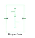
Gear ratio 10

Represents a fixed-ratio gear or gear box. No inertia or compliance is modeled in this block. You can optionally include gear meshing and viscous bearing losses.

Connections B (base) and F (follower) are mechanical rotational conserving ports. Specify the relation between base and follower rotation directions with the Output shaft rotates parameter. Optionally include thermal effects and expose thermal conserving port H by right-clicking on the block and selecting Simscape block choices to switch between variants.

output shaft rotates in the same direction of the motor output.

Base is connected to the Motor shaft and the follower is connected to the Rear wheel drive.

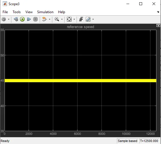
Drive cycle of the electric rickshaw for 100 km at 45 KMPH.

So to cover 100 km with speed of 45 kmph we required 12500 sec .

Excel sheet for input and assumed data

RESULTS.

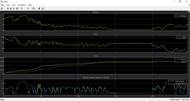
1.FTP 75 drive cycle

Here we can see the results of the model with FTP 75 drive cycle .

first plot is about energy

energy consumption is from 0 to -10 KWH

second plot is SOC

SOC% is reduced 100 to 80 %

Third plot is temperature , temp1 is for controller and temp2 is for motor

temperature of controller is high than the temperature of motor

Fourth plot is velocity of vehicle speed and Drive cycle(reference).

vehicle speed is not exactly equal to the reference speed due to inertia and losses .

2.WOT DRIVE cycle

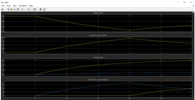
first plot is about energy

energy consumption is from 0 to -10 KWH

second plot is SOC

SOC% is reduced 100 to 80 %

Third plot is temperature , temp1 is for controller and temp2 is for motor

temperature of controller is high than the temperature of motor

Fourth plot is velocity of vehicle speed and Drive cycle(reference).

vehicle speed is not exactly equal to the reference speed due to inertia and losses

3.Manually prepared drive cycle

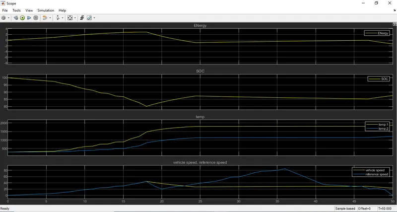
Here we can see the results of the model with manual drive cycle .

first plot is about energy varys from 0 to 2.

second plot is SOC is varys between 100 % to 80 %

Third plot is temperature , temp1 is for controller and temp2 is for motor . temperature of the co

Fourth plot is velocity of vehicle speed and Drive cycle(reference). Up to 18 secs both are same but after 18 seconds both speeds get differ.

4.Constant speed drive cycle

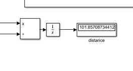
Here we can see the distance travelled by the electric rickshaw in the display , we can see in the below fig.

Here we can see the results of the model with constant drive cycle .

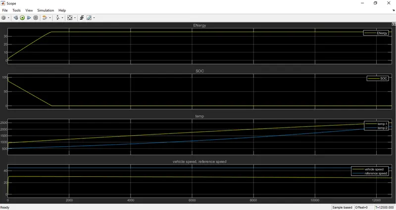
first plot is about energy

Energy consumption from 0 to 35, than 35 constant energy consumption

second plot is SOC

SOC is reduced to 100% to 0%

Third plot is temperature , temp1 is for controller and temp2 is for motor

temperature of controller is higher than temperature of motor .

Fourth plot is velocity of vehicle speed and Drive cycle(reference).

Here we can see that the reference speed is 45 kmph but we getting speed of the vehicle is 30 kmph due to parameters losses.