Final Project: Electric Rickshaw modelling

Objective:

• In this project, we are going to build the MATLAB model of the E-Rickshaw using a PM brushed type DC motor.
• We come to know what is E-Rickshaw and how it works and the benefits of this vehicle.
• Then we make an E-Rickshaw by using MATLAB and SIMULINK software.
• For three standard driving cycles energy consumption, temperature rise of motor and controller for 100 km constant speed driving at 45 kmph

Introduction:

• The popularity of Autorickshaw among Indians is such that it is a medium of commutation for the normal man. About 1.5 million battery-powered, three-wheeled rickshaws – a fleet bigger than the total number of electric passenger cars sold in China since 2011.
• As many as 11,000 new e-rickshaws hit the streets every month, and annual sales are expected to increase about 9 percent by 2021, according to consulting firm A.T. Kearney. Three-wheeled vehicles make up a $1.5 billion market, and manufacturers of electric versions include Mahindra & Mahindra Ltd and Kinetic Engineering Ltd, along with smaller outfits that assemble parts imported from China.
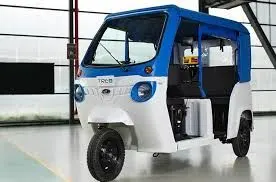
• An attempt has been made to model Mahindra treo electric rickshaw. The Mahindra Treo is aimed to be a clean and silent mobility solution for the city. The design remains identical to a conventional three-wheeler or what we dearly call an auto-rickshaw which is a popular choice among Indians. The Mahindra Electric Treo is powered by a 7.47kWh Li-ion battery which makes 5.4kW and 30Nm of torque. The battery can be charged to its full capacity in three hours and 50 minutes. The driving range is claimed to be 170 kilometers and has a top speed of 45km/h.
  
  
• 
• Since data like the coefficient of drag, rolling resistance, and gear ratios the data was taken from a BAJAJ RE model which is similar to treo from a paper titled "Modelling, design, and control of a light electric vehicle with hybrid energy
  storage system for Indian driving cycle".
• Vehicle dynamic modelling-By using Newton’s law of motion, the vehicle is modeled as a load by considering various longitudinal forces acting on it.
• 
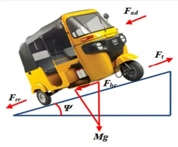
• The tractive force, Ft, required to drive the wheels by overcoming resistive force is given by Ft = Frr + Fad + Fhc +Fla +Fva, where Frr is the rolling resistance force, Fad is the aerodynamic drag, Fhc is the hill-climbing force, Fla is the
  linear acceleration force and Fva is the rotational acceleration force
• Using the obtained instantaneous tractive forces and the speed of the vehicle, the tractive power required at wheels is calculated as
  Tractive power, Pt = Ft*v

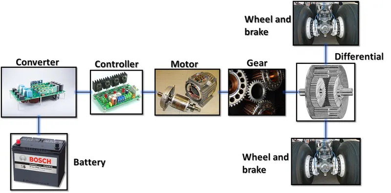
Block diagram of powertrain:

Model:

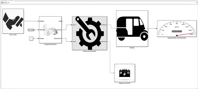
Drive cycle :

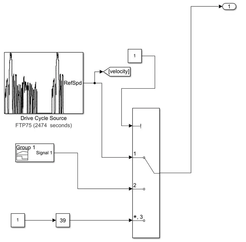
The Drive Cycle Source block generates a standard or user-specified longitudinal drive cycle. The block output is the specified vehicle longitudinal speed.

1. drive cycle source(FTP75): this is the Matlab built-in drive cycle that gives desired output speed to the driver which compares this with the current speed and produces an error.
2. signal builder: this drive cycle is made by the user by choosing the appropriate speed he wants at the instant.
3. slider gain: using this block you can control the speed of the vehicle by adjusting the slider.

here, The Multiport Switch block determines which of several inputs to the block passes to the output. The block bases this decision on the value of the first input. The first input is the control input and the remaining inputs are the data inputs. The control input value determines which data input passes to the output.

Driver:

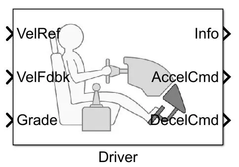
Inputs:

• VelRef: takes the input from the drive cycle.
• VelFdbk: takes the input from the velocity of the vehicle and compares it with the reference velocity here there will be an error signal if the signal is a positive error then the driver block will give a signal to the accelCmd to increase and vice versa.
• Grade: indicates the % of the gradeability i.e the angle of slope.
• AccelCmd: this output is given to the controlled PWM voltage to process the PWM signal, which is connected to the H-bridge input PWM to control speed and torque.
• DecelCmd: this output is directly given to the BRK input of the H-bridge.

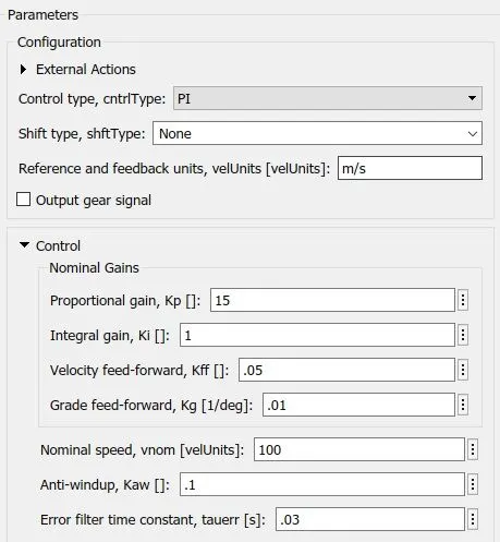
A parametric longitudinal speed tracking controller for generating normalized acceleration and braking commands based on reference and feedback velocities.

Use the external actions to input signals that can disable, hold, or override the closed-loop commands determined by the block. The block uses this priority for the input commands: disable, hold, override.

Motor and Controller Subsystem:

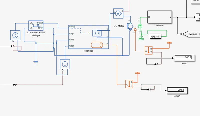
The input to this system is given by the longitudinal driver the two inputs are acceleration and deceleration command depending upon the desired speed and torque.

• acceleration command input is given to controlled PWM voltage via a controlled voltage source to process the PWM signal, which is connected to the H-bridge input PWM to control speed, and torque
• deceleration command is directly given to the BRK input of the H-bridge via controlled voltage source.
• solver configuration block specifies the solver parameters that your model needs before you can begin the simulation. Each topologically distinct Simscape block diagram requires exactly one Solver Configuration block to be connected to it.
• H-bridge is connected here this is a power converter that regulates voltage to control the speed and torque of the DC motor and hence the two terminals are connected to the motor as shown above.
• The Current Sensor block represents an ideal current sensor, that is, a device that converts current measured in any electrical branch into a physical signal proportional to the current. Connections + and – are electrical conserving ports through which the sensor is inserted into the circuit. The connection is a physical signal port that outputs the measurement result.
• the current sensor output is given to the battery subsystem.
• the DC-motor output is given to the vehicle body i.e the power is given to the transmission and gear system to perform the desired condition.

H-Bridge

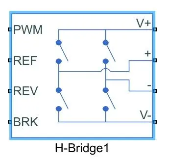
This block represents an H-bridge motor drive. The block can be driven by the Controlled PWM Voltage block in PWM or Averaged mode. In PWM mode, the motor is powered if the PWM port voltage is above the Enable threshold voltage. In Averaged mode, the PWM port voltage divided by the PWM signal amplitude parameter defines the ratio of the on-time to the PWM period. Using this ratio and assumptions about the load, the block applies an average voltage to the load that achieves the correct average load current. The Simulation mode parameter value must be the same for the Controlled PWM Voltage and H-Bridge blocks.

If the REV port voltage is greater than the Reverse threshold voltage, then the output voltage polarity is reversed. If the BRK port voltage is greater than the Braking threshold voltage, then the output terminals are short-circuited via one bridge arm in series with the parallel combination of a second bridge arm and a freewheeling diode. Voltages at ports PWM, REV, and BRK are defined relative to the REF port.

DC-motor:

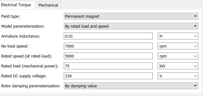
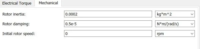
This block represents the electrical and torque characteristics of a DC motor. The block assumes that no electromagnetic energy is lost, and hence the back-emf and torque constants have the same numerical value when in SI units. Motor parameters can either be specified directly or derived from the no-load speed and stall torque. If no information is available on armature inductance, this parameter can be set to some small non-zero value. When a positive current flows from the electrical + to - ports, a positive torque acts from the mechanical C to R ports. Motor torque direction can be changed by altering the sign of the back-emf or torque constants.

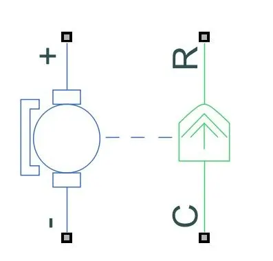
The resulting torque across the block is:

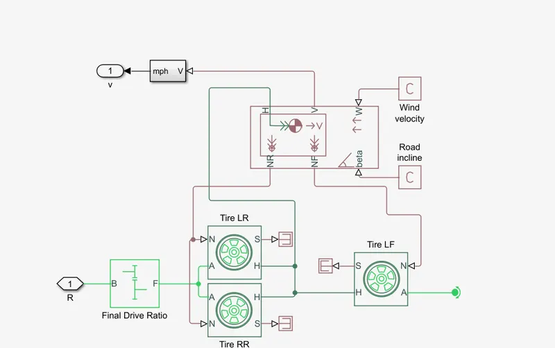
• the gears are connected to the wheels' transmission.
• the tire hubs are connected to the vehicle body.
• this vehicle is a rear-wheel drive and hence the power that is transmitted through gears is given to the real tired only.
• a moment inertia block is also given to the gear system since there will be initial inertia during the start of the vehicle.

vehicle body:

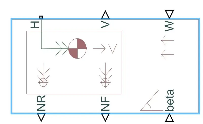
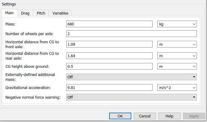
Represents a two-axle vehicle body in longitudinal motion. The block accounts for body mass, aerodynamic drag, road incline, and weight distribution between axles due to acceleration and road profile. The vehicle can have the same or different wheels on each axle. Optionally include pitch and suspension dynamics or additional variable mass and inertia. The vehicle does not move vertically relative to the ground.

Connection H is the mechanical translational conserving port associated with the horizontal motion of the vehicle body. The resulting traction motion developed by tires should be connected to this port. Connections V, NF, and NR are physical signal output ports for vehicle velocity and front and rear normal wheel forces. Wheel forces are considered positive if acting downwards. Connections W and beta are physical signal input ports corresponding to headwind speed and road inclination angle. If the variable mass is modeled, the physical signal input ports CG and M are exposed. CG accepts a two-element vector representing the x and y distance offsets from vehicle CG to additional load mass CG. M represents the additional mass. If both variable mass and pitch dynamics are included, the physical signal port J accepts the inertia of the additional mass about its own CG.

Tire:

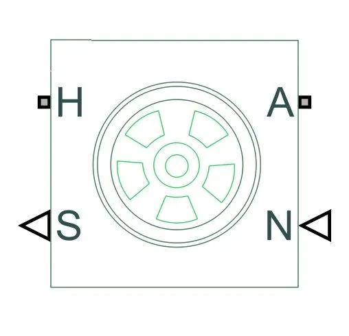
Represents the longitudinal behavior of a highway tire characterized by the tire Magic Formula. The block is built from Tire-Road Interaction (Magic Formula) and Simscape Foundation Library Wheel and Axle blocks. Optionally, the effects of tire inertia, stiffness, and damping can be included.

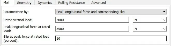
Connection A is the mechanical rotational conserving port for the wheel axle. Connection H is the mechanical translational conserving port for the wheel hub through which the thrust developed by the tire is applied to the vehicle. Connection N is a physical signal input port that applies the normal force acting on the tire. The force is considered positive if it acts downwards. Connection S is a physical signal output port that reports the tire slip. Optionally expose physical signal port M by setting Parameterize by to Physical signal Magic Formula coefficients. Physical signal port M accepts a four-element vector corresponding to the B, C, D, and E Magic Formula coefficients.

Battery and SOC Subsystem:

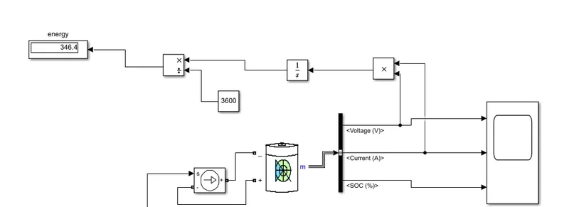
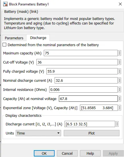
for the power source, we have used a battery source block which disconnected to a constant block. When we double click on Battery block we get the following box

SOC Estimate:

Estimates the batter SOC% using the coulomb counting method for 100km. It takes current as the input and gives SOC% as output. The initial SOC of the battery is assumed to be 100%. And while calculating the SOC, battery capacity is assumed to be 100Ah.

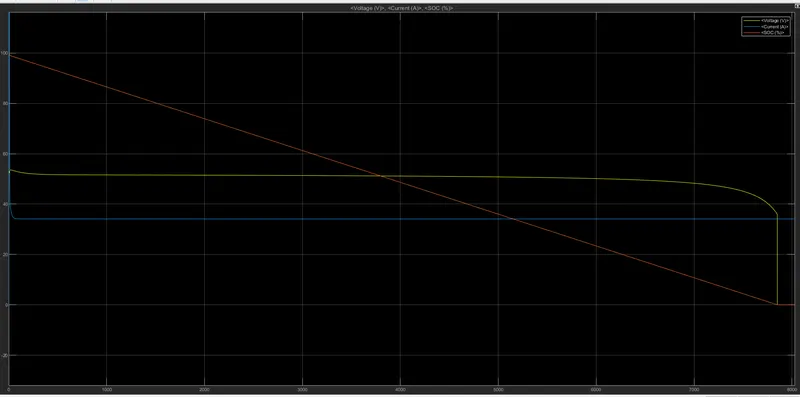
and it it clear from the above plot that model can run exactly for 100km and hence the range of the vehicle is 100km because SOC is zero at the end of 100km run.

Simulation and its results:

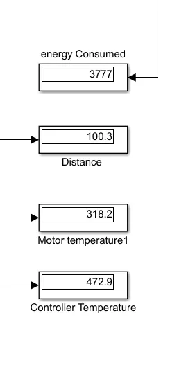
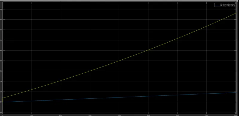
For 100 km constant speed driving at 45 kmph.

energy consumption: 3777 joules

temperature rise of motor and controller: 318.3 K and 472.9K respectivley

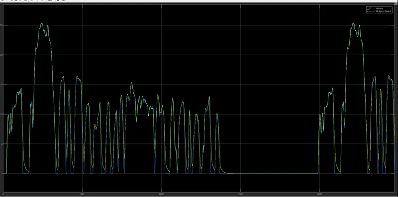
The FTP75 drive cycle is given as a speed reference to the driver. The FTP cycle (for Federal Test Procedure) has been created by US EPA (Environmental Protection Agency) to represent a commuting cycle with a part of urban driving including frequent stops and a part of highway driving. this cycle covers a distance of 17.77 Km in 2474 seconds. note it has a top speed of 90km/hr

Run time is 2472 seconds:

the below image shows the reference speed or the desired speed of the drive cycle and the vehicle actual speed with respect to time. Achieved using the model.

Model file link (Click here)