Final Project: Electric Rickshaw modelling
Objective:
To develop a detailed MATLAB model of an electric rickshaw with rear wheels driven by a PM brushed motor. To Incorporate motor controller and motor efficiency points and to create an Excel sheet with input and assumed data. To analyze energy consumption and temperature rise for 100 km constant-speed driving at 45 kmph, using three standard driving cycles. Assumed Efficiency of motor and controller as 100%.
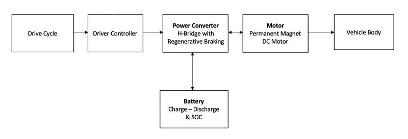
Block Diagram:
E-Rickshaw Vehicle Power Calculations:
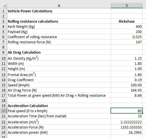
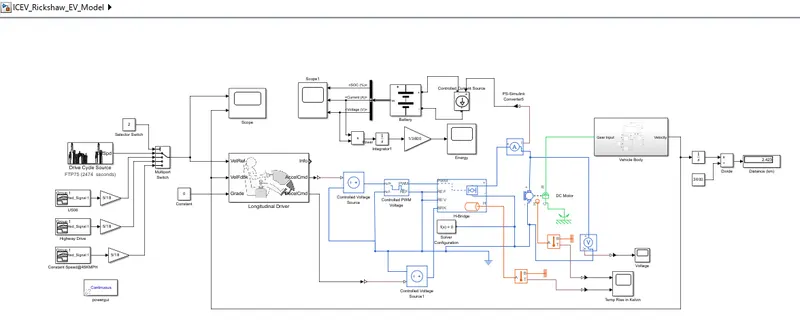
The electric vehicle model is designed in the Matlab simulink environment to simulate and test the performance based on the calculated values. The main components that is used to build an EV model is listed below:
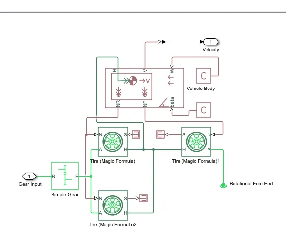
- Vehicle Body, Tires and simple gear system
- DC motor Block (Permanent magnet type)
- Isolation circuit i.e., H-Bridge
- Controlled PWM voltage block connected with controlled voltage source block
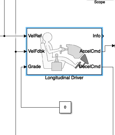
- Longitudinal Driver block
- Drive cycle source
Vehicle Body Subsystem:
The vehicle body subsystem consists of Vehicle Body, Tires and simple gear system as shown below:
Vehicle Body Block:
H input port:
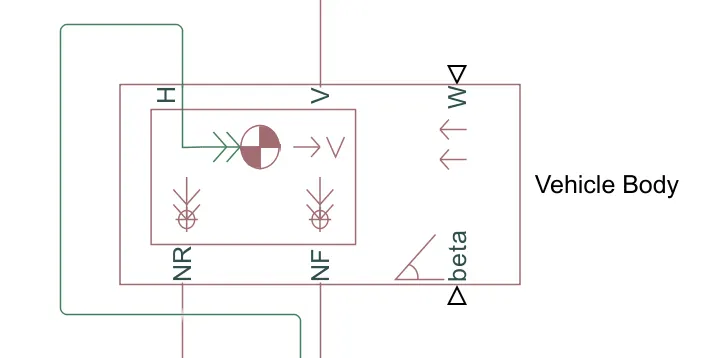
It is the Hub (H) of the vehicle body where Hub (H) of the tire is connected.
V output port:
It gives the actual velocity of the vehicle.
NR and NF output Port:
NF and NR are the normal forces acting on the front and real wheels respectively.
W input Port:
W input port takes the wind velocity as input and it which is not considered in my model
Beta Input port:
Beta input port takes inclination or hill climbing angle as an input which is not considered in my model.
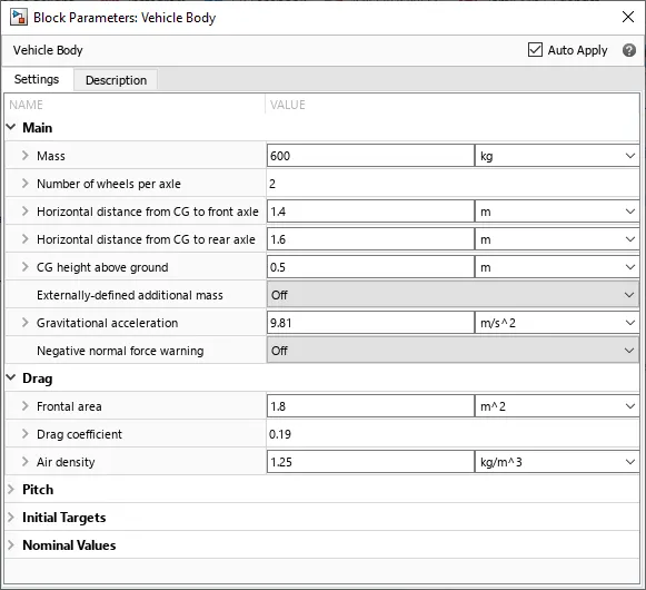
Parameters of vehicle body block:
Tire Block:
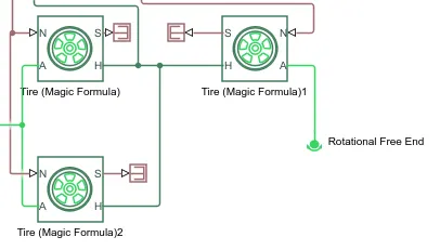
H input port :
It represents the hub of the wheel and all the wheel hubs are connected together.
A input port:
It represents the axle of the wheel, Two tire A port are connected together to form a front axle and another Two tire A port are connected together to form a rear axle, the rear axle is further connected with the output shaft of the gear mechanism which transfers power to the wheel.
N input port:
It represent the normal forces acting on the wheel and the front axle pair of wheel takes input from the NF port of vehicle body and the rear axle pair of wheel takes input from the NR port of the vehicle body.
S output port:
It represents the slip of the tire and it is not considered in my model.
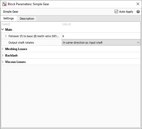
Simple Gear Block:
It represents a fixed-ratio gear or gear box. No inertia or compliance is modeled in this block.
Connections B (base) is the input port which is connected with the motor shaft and F (follower) are connected with the axle of the rear wheel.
Dc Motor Block:
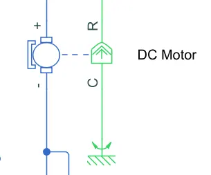
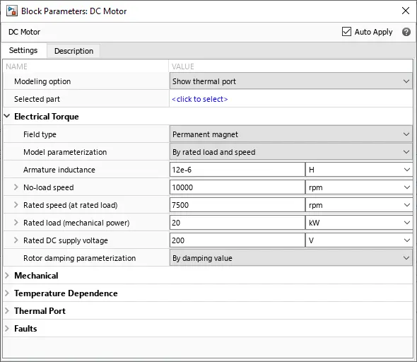
This block represents the electrical and torque characteristics of a DC motor.
The block parameters which is set on the model is shown below:
ISOLATION CIRCUIT:
The H-Bridge block serves as a isolation circuit between the electric and electronic components.
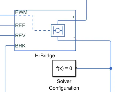
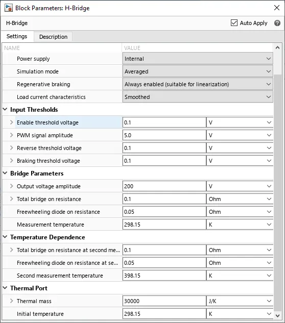
This block represents an H-bridge motor drive. The block can be driven by the Controlled PWM Voltage block in PWM or Averaged mode. In PWM mode, the motor is powered if the PWM port voltage is above the Enable threshold voltage. In Averaged mode, the PWM port voltage divided by the PWM signal amplitude parameter defines the ratio of the on-time to the PWM period. Using this ratio and assumptions about the load, the block applies an average voltage to the load that achieves the correct average load current. The Simulation mode parameter value must be the same for the Controlled PWM Voltage and H-Bridge blocks.
Block Parameters:
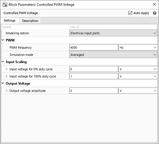
Controlled PWM Voltage:
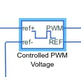
This block creates a Pulse-Width Modulated (PWM) voltage across the PWM and REF ports. The output voltage is zero when the pulse is low, and is equal to the Output voltage amplitude parameter when high. Duty cycle is set by the input value.
Block Parameters:
Longitudinal Driver Block:
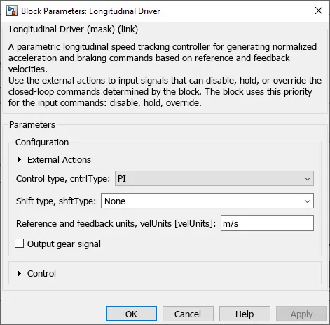
A parametric longitudinal speed tracking controller for generating normalized acceleration and braking commands based on reference and feedback velocities.
Block Prameters:
Drive Cycle Source Block:
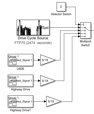
Generates a standard or user-specified longitudinal drive cycle. The block output is the vehicle longitudinal speed. we can import drive cycles from:
- Predefined sources
- Workspace variables, including arrays and time series objects
- mat, xls, xlsx, or txt files
Use the fault tracking parameters to identify drive cycle faults within specified speed and time tolerances.
Simulink Model:
Scope Outputs:
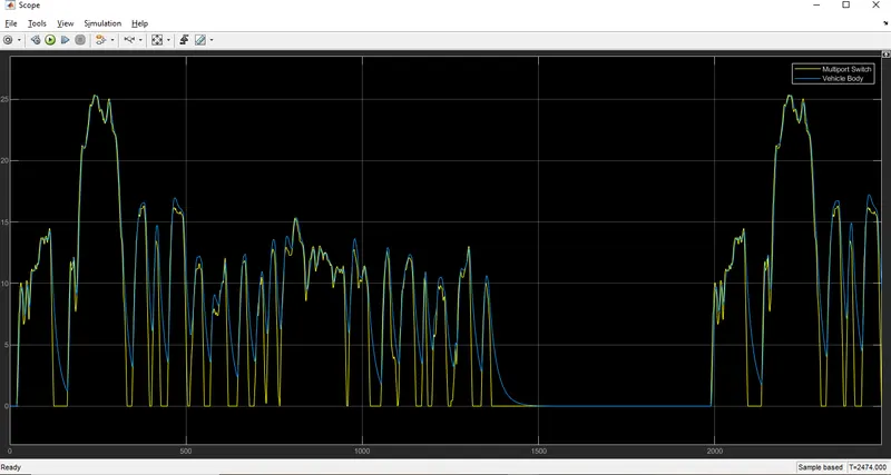
Vehicle response for FTP75 DriveCycle
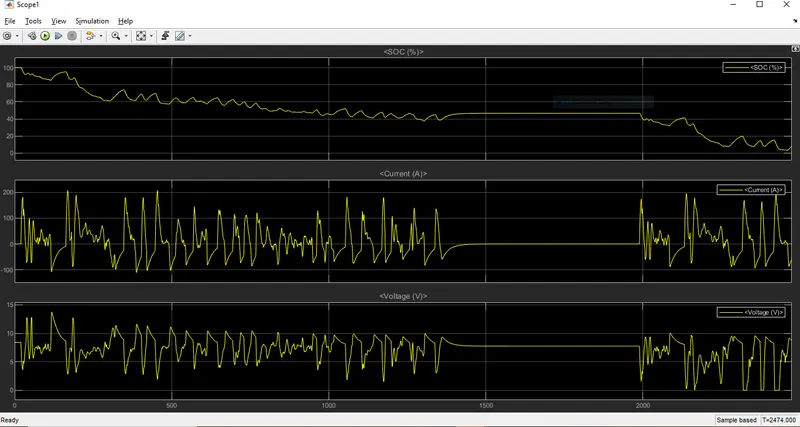
Effect on Battery (SOC, Voltage and current) for FTP75 Drive Cycle:
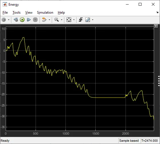
Energy Consumed for FTP75 DriveCycle:
Temperature Rise on Motor and H-Bridge for FTP75 Drive Cycle:
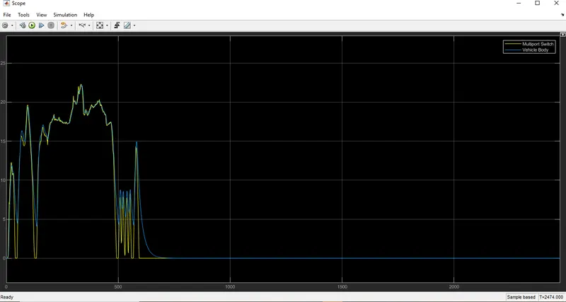
Vehicle response for US06 Drive Cycle:
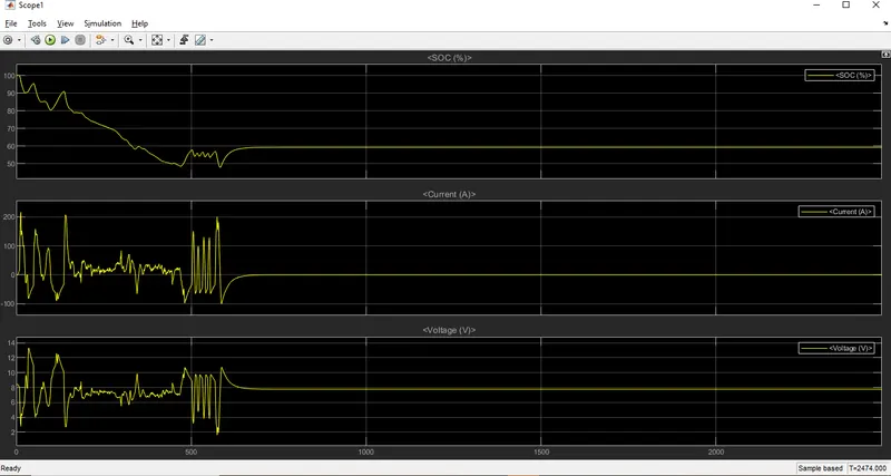
Effect on battery (SOC, Voltage and current) for US06 Drive Cycle:
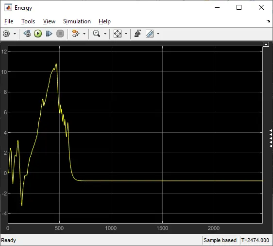
Energy Consumed for US06 DriveCycle:
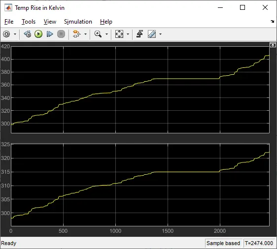
Temperature Rise on Motor and H-Bridge for US06 Drive Cycle:
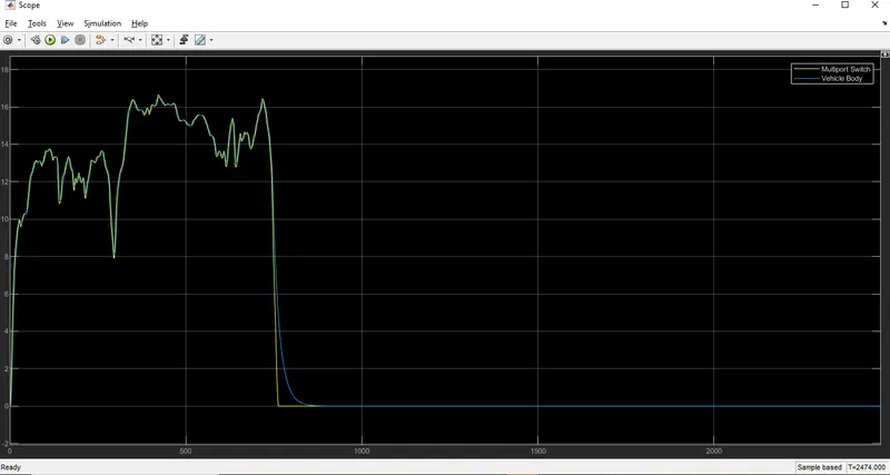
Vehicle response for Highway Drive Cycle:
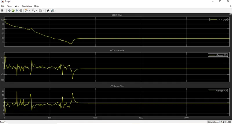
Effect on battery (SOC, Voltage and current) for Highway Drive Cycle:
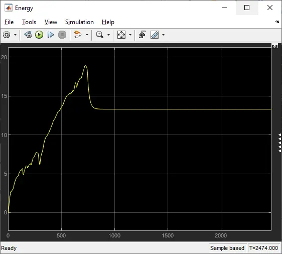
Energy Consumed for Highway Drive Cycle:
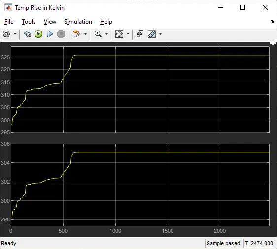
Temperature Rise on Motor and H-Bridge for Highway Drive Cycle:
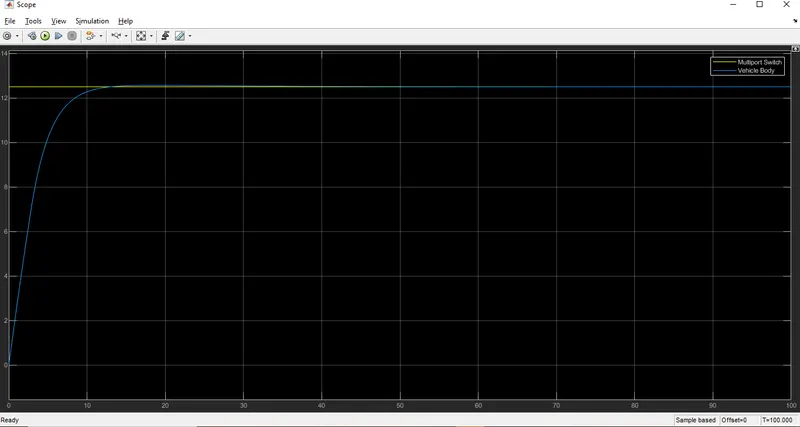
Vehicle response for Constant speed drivecycle at 45kmph for 100 seconds:
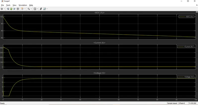
Effect on battery (SOC, Voltage and current) for Constant speed drivecycle at 45kmph for 100 seconds:
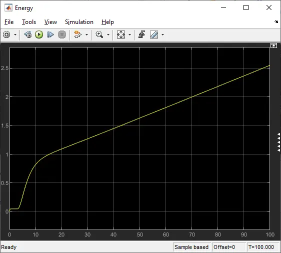
Energy Consumed for Constant speed drivecycle at 45kmph for 100 seconds:
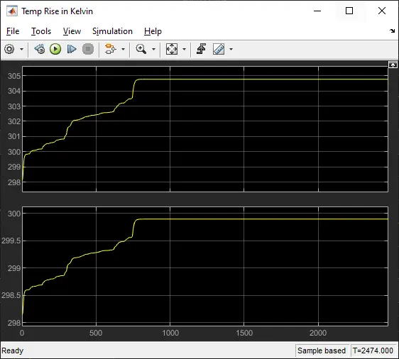
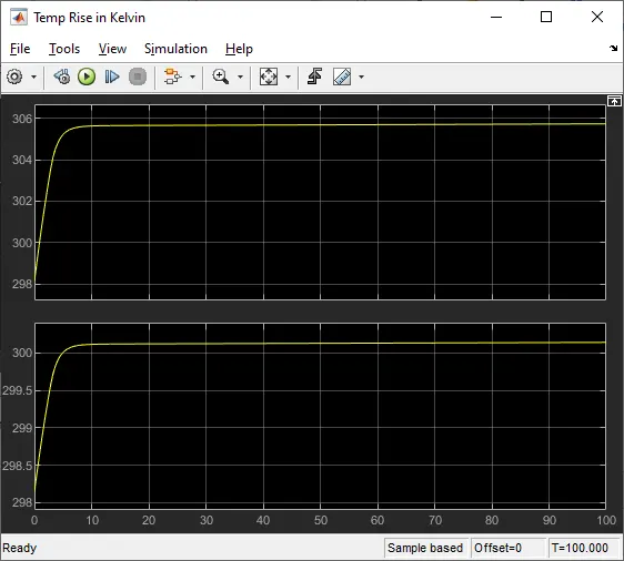
Temperature Rise on Motor and H-Bridge for Constant speed drivecycle at 45kmph for 100 seconds:
Conclusion:
EV model is designed with the calculated values in MATLAB simulink environment, ran the simulation for all the drive cycles and observed the results of the vehicle body velocity and reference velocity i.e drive cycle and found that model is able to trace the drive cycle velocity. Also observed the discharge - charge & SOC of the battery throughout the drive cycle and found battery is getting charged during deceleration of the vehicle through regenerative braking. Also observed Energy consumption and temperature rise of the motor and Isolation Circuit.