Electric Rickshaw modelling in SIMULINK
AIM -
Create a detailed MATLAB model of an electric rickshaw (three-wheel passenger vehicle) as per the details below:
- Rear wheels driven by PM brushed type motor
- Assume efficiency points of motor controller and motor
- Make an excel sheet of all input and assumed data
Results: For any three standard driving cycles show energy consumption, the temperature rise of motor and controller
EXPLANATION -
Electric rickshaws have been becoming more popular in some cities since 2008 as an alternative to auto rickshaws and pulled rickshaws because of their low fuel cost, and less human effort compared to pulled rickshaws. They are being widely accepted as an alternative to petrol/diesel/CNG auto-rickshaws. They are three-wheelers powered by an electric motor ranging from 650 to 1400 Watts. They are mostly manufactured in India and China, only a few other countries manufacture these vehicles. Battery-run rickshaws could be a low-emitter complimentary transport for the low-income people, who suffer most from a lack of transport facility if introduced systematically according to experts.
These rickshaws have an M.S(Mild Steel) tubular Chassis, consisting of three wheels with a differential mechanism at the rear wheels. The motor is a brushless DC motor manufactured mostly in India and China. The electrical system used in the Indian version is 48V and in Bangladesh is 60V. The body design from the most popular Chinese version is of very thin iron or aluminum sheets. Vehicles made in fiber are also popular because of their strength and durability, resulting in low maintenance, especially in India. The body design is varied from load carriers, passenger vehicles with no roof, to full body with windshield for drivers comfort. It consists of a controller unit. They are sold based on the voltage supplied and current output, also the number of MOSFET (metal oxide field-effect transistors) used. The battery used is mostly a lead-acid battery with a life of 6–12 months. Deep cycle batteries designed for electric vehicles are rarely used. The weight of the electric car has also been a recurring design difficulty in them.
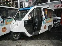
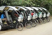
Let us look into Mahendra's first low-maintenance Lithium-ion battery-powered 3-wheeler whose parameters will be used in our Simulink model.
Mahindra Treo is a revolutionary new range of electric autos, e-rickshaw, and cargo versions. It is powered by advanced Lithium-ion technology which offers higher savings, superior ride quality, and best-in-class interior space.
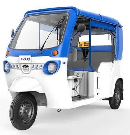
The specification sheet of Mahendra Treo is shown below -
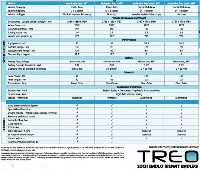
Specifications of Mahendra Treo - HRT version, which is a D+3 seater -
1. Battery type, Voltage - Lithium-ion, 48V
2. Battery capacity (Installed) - 7.37 kWh
3. Charging Time 0-100% at standard conditions - 3h 50 min
4. Peak power - 8 kW
5. Peak torque - 42 Nm
6. Transmission type - Direct drive
PROCEDURE FOR MAKING A SIMULINK MODEL OF AN ELECTRIC RICKSHAW -
First, let us look into the drivetrain of a basic electric rickshaw.
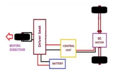
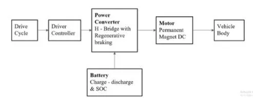
Similar to the above image, we will be modeling a rear-wheel drive electric rickshaw. The vehicle body will be connected with a permanent magnet DC motor (as required). This DC motor will then be connected to the power converter which in turn will be connected to the driver controller which gives the acceleration pedal command to the power converter. The input data to the model will be given in the form of a drive cycle.
This can be explained in the form of a block diagram and we will be following the same while designing it.
Building the vehicle body in Simulink -
We will look into the different Simulink blocks used in creating the vehicle body for our electric rickshaw.
The below image shows us the complete subsystem of the vehicle body which is created for our model -
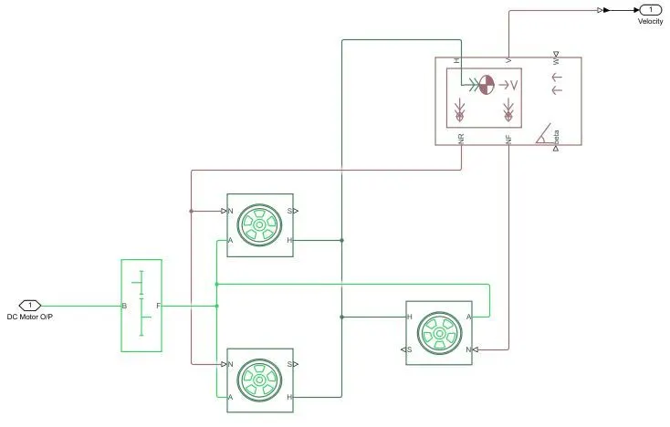
From the above image, we can see that various blocks have been used. The theory behind these blocks and the parameters that are used will be explained below.
1. Tire (Magic Formula)
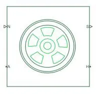
The Tire (Magic Formula) block models a tire with longitudinal behavior given by the Magic Formula, an empirical equation based on four fitting coefficients. The block can model tire dynamics under constant or variable pavement conditions.
The longitudinal direction of the tire is the same as its direction of motion as it rolls on the pavement. This block is a structural component based on the Tire-Road interaction (Magic Formula) block.
To increase the fidelity of the tire model, we can specify properties such as tire compliance, inertia, and rolling resistance. However, these properties increase the complexity of the tire model and can slow down the simulation.
It has the following ports-
1. Input port, N - Normal force acting on the tire, it is positive when force is acting downwards/towards the surface.
2. Output port, S - Slip value relative to tire and surface of contact.
3. Conserving port, H - represents wheel hub which transmits thrust generated by the wheel to the body of the vehicle.
4. Conserving port, A - represents the axle on which the tires are mounted.
Tire parameters -
The default values will be considered for the parameters and are shown below.
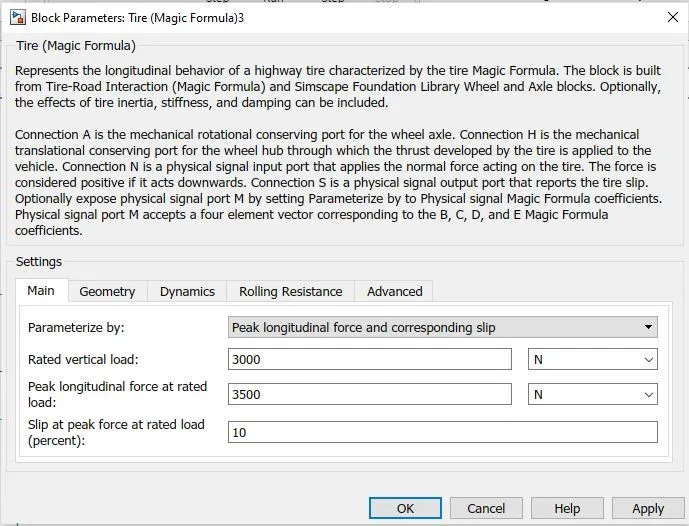
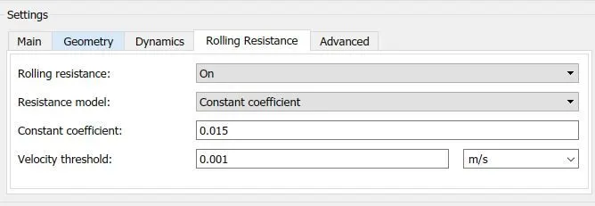
The Rolling resistance will be turned on and the default value will be considered.
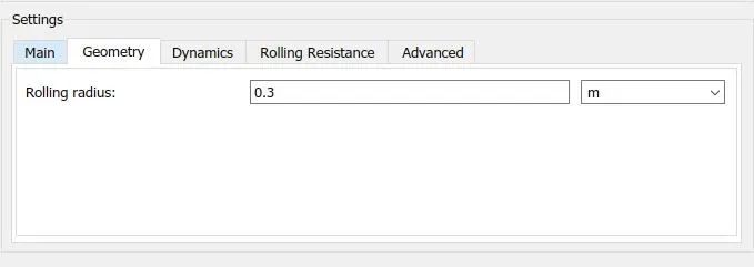
The other parameters are shown below.
2. Vehicle Body -
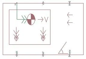
The Vehicle Body block represents a two-axle vehicle body in longitudinal motion. The vehicle can have the same or a different number of wheels on each axle. For example, two wheels on the front axle and one wheel on the rear axle. The vehicle wheels are assumed identical in size. The vehicle can also have a center of gravity (CG) that is at or below the plane of travel.
The block accounts for body mass, aerodynamic drag, road incline, and weight distribution between axles due to acceleration and road profile. Optionally include pitch and suspension dynamics. The vehicle does not move vertically relative to the ground.
The block has an option to include an externally defined mass and externally defined inertia. The mass, inertia, and center of gravity of the vehicle body can vary over the course of simulation in response to system changes.
It has the following ports -
1. Input port, W - wind velocity in m/s
2. Input port, beta - Grade angle in radians
3. Output port, V - Velocity in m/s
4. Output port, NR - Normal force on Rear axle (N)
5. Output port, NF - Normal force on front axle (N)
Vehicle body Parameters -
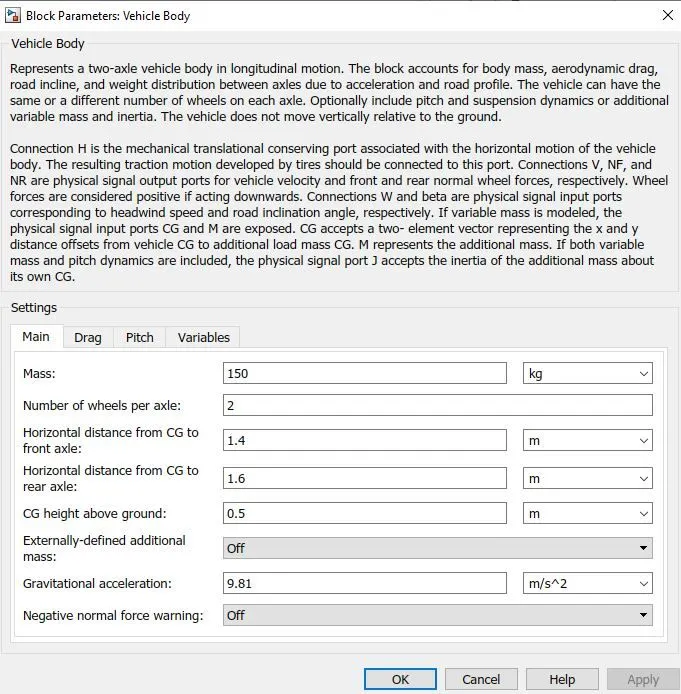
1. The Vehicle mass = 150 kg (Will be taking this value to achieve the proper results)
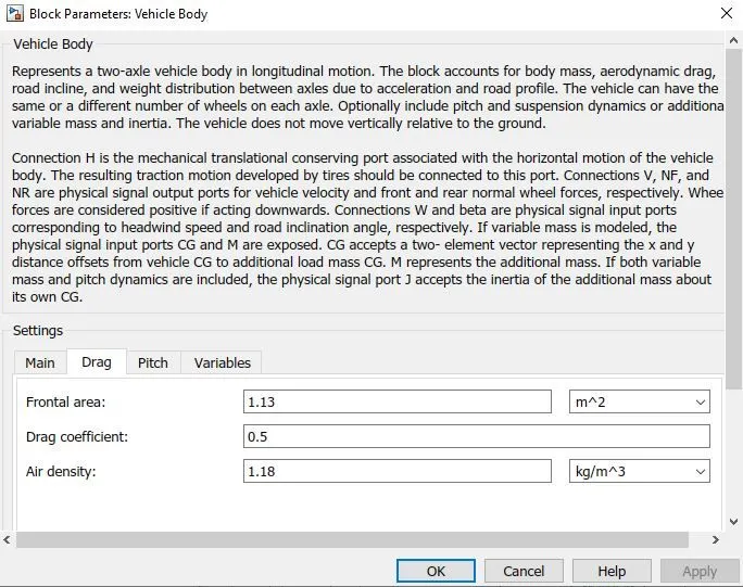
2. Frontal area = 1.13m^2
3. Drag coefficient = 0.5
4. Air density = 1.18 kg/m^3
5. Gravitational acceleration = 9.81 m/s
The below images shows the defined parameters along with the default ones.
3. Simple gear -
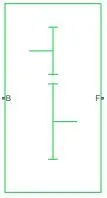
The Simple Gear block represents a gearbox that constrains the connected driveline axes of the base gear, B, and the follower gear, F, to corotate with a fixed ratio that you specify. You choose whether the follower axis rotates in the same or opposite direction as the base axis. If they rotate in the same direction, the angular velocity of the follower, ωF, and the angular velocity of the base, ωB, have the same sign. If they rotate in opposite directions, ωF and ωB have opposite signs.
The ports are explained below -
1. B - the output of B, base gear is connected with the input of DC motor R. It is a rotational mechanical conserving port.
2. F - The output of the F, follower gear is connected with the rear axle. It is also a rotational mechanical conserving port.
We will use the parameters shown below.
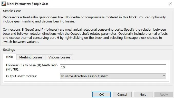
With the implementation of the above blocks, we create a subsystem in Simulink which acts as a vehicle body for our electric rickshaw.
We won't be adding the wind velocity and grade angle values to the vehicle body as it will increase our simulation time. We will also ignore the slip value in the tires to simplify our simulation.
BUILDING THE MOTOR AND POWER CONTROL SYSTEM -
We will now look into the different Simulink blocks used in creating the motor and power control system for our electric rickshaw.
The below image shows us the complete system which is created for our model -
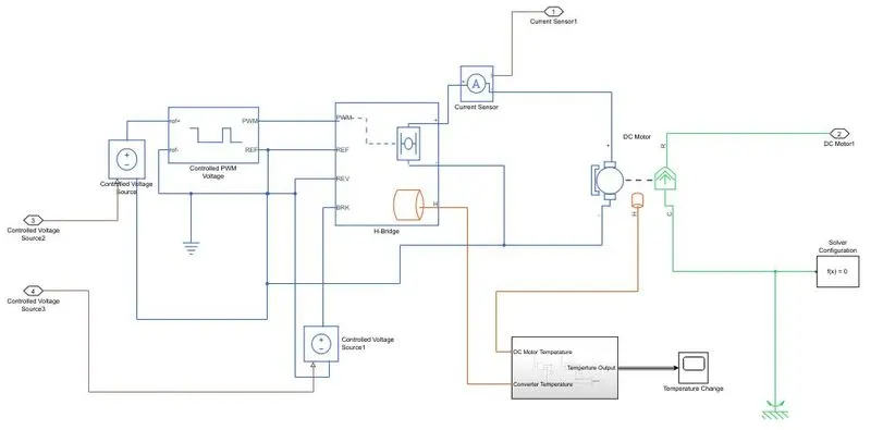
1. DC motor -
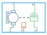
The DC Motor block represents the electrical and torque characteristics of a DC motor using the following equivalent circuit model:
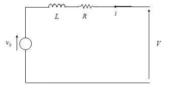
We can specify the equivalent circuit parameters for this model when you set the Model parameterization parameter to 'By equivalent circuit parameters'. The resistor R corresponds to the resistance you specify in the Armature resistance parameter. The inductor L corresponds to the inductance you specify in the Armature inductance parameter. You can specify how to generate the magnetic field of the DC motor by setting the Field type parameter to the desired option.
The ports are explained below -
1. + - Ports receiving electrical signals associated with the motor positive terminal
2. - - Ports receiving electrical signals associated with the motor negative terminal
3. C - Mechanical conserving port associated with the casing of the motor and is connected to a mechanical rotational reference block.
4. R - Mechanical conserving port associated with Rotor shaft of the motor which produces required input to the transmission system.
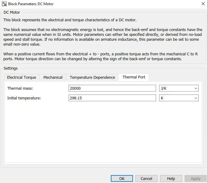
5. Thermal port - The block has an optional thermal port, hidden by default. To expose the thermal port, right-click the block in your model, and then from the context menu select Simscape > Block choices > Show thermal port. This action displays the thermal port H on the block icon and exposes the Temperature Dependence and Thermal Port parameters.
DC motor Parameters -
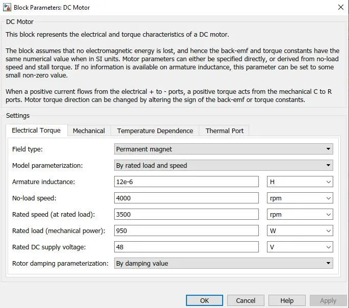
The rated load is changed to 950 W, the rated DC supply voltage is 48 V, the no-load speed is changed to 4000 rpm and the rated speed is changed to 3500 rpm. The motor is of permanent magnet type as per requirement.
The rest of the parameters are default and are shown below.
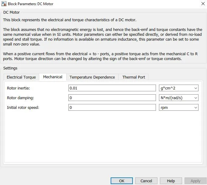
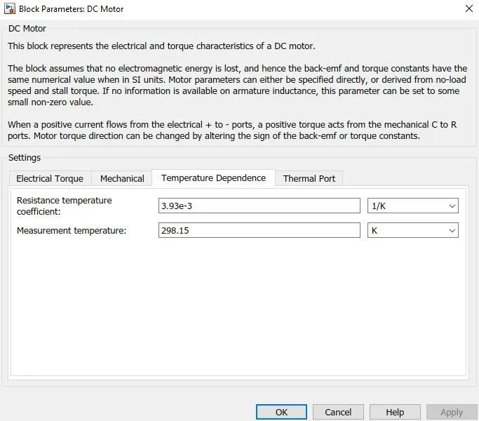
The thermal port will be made visible so that we can observe the temperature change in the DC motor and the controller during its operation.
2. H-Bridge -
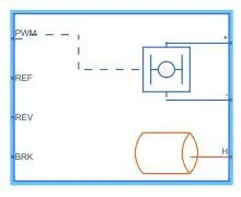
H-Bridge block is used to represent the H-Bridge motor driver which controls the power input to the motor according to the load requirements. The output provided by the block is controlled voltage depending on the control signal.
The ports are explained below -
1. + - conserving port associated with the positive load connection usually connected to positive port of the motor.
2. - - conserving port associated with the negative load connection usually connected to the negative terminal of the motor.
3. PWM - conserving port associated with PWM control signal (voltage pulses)
4. REF - Conserving port associated with a zero voltage reference.
5. REV - conserving port associated with voltage controlling polarity change of bridge output signal.
6. BRK - conserving port associated with voltage when brakes are applied, thereby aiding the process of regenerative braking.
7. Thermal port - The block has an optional thermal port, hidden by default. To expose the thermal port, right-click the block in your model, and then from the context menu select Simscape > Block choices > Show thermal port. This action displays the thermal port H on the block icon and adds the Temperature Dependence and Thermal Port parameters.
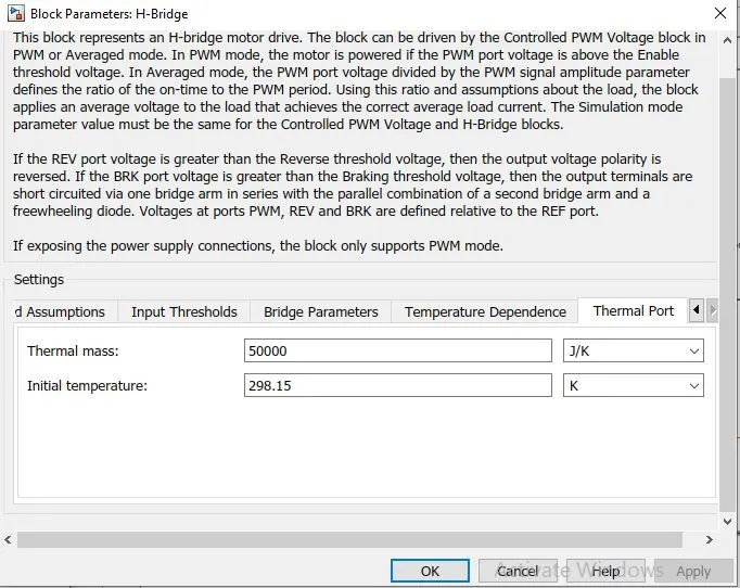
H-bridge parameters -
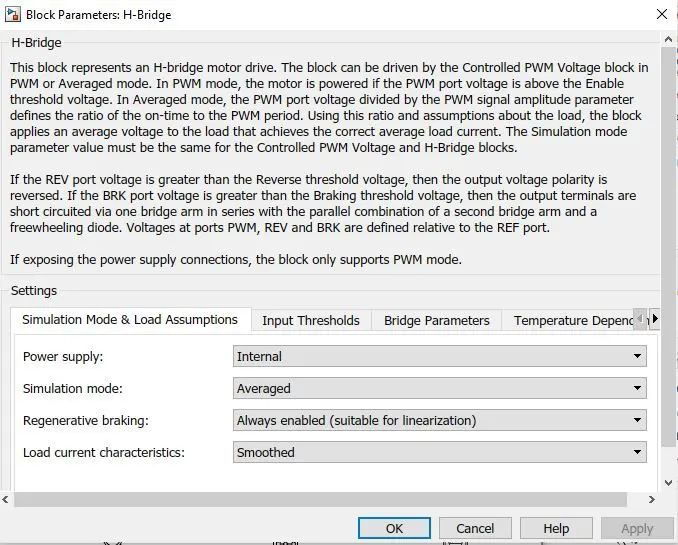
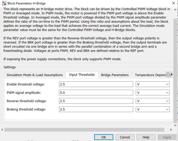
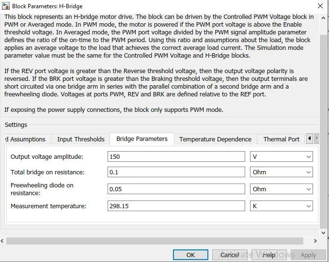
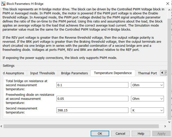
The default parameters will be used in this model for the H-bridge block as shown below.
3. Controlled PWM Voltage -
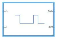
The Controlled PWM Voltage block represents a pulse-width modulated (PWM) voltage source. The block has two modeling variants, accessible by right-clicking the block in your block diagram and then selecting the appropriate option from the context menu, under Simscape > Block choices:
- Electrical input ports — The block calculates the duty cycle based on the reference voltage across its ref+ and ref- ports. This modeling variant is the default.
- PS input — Specify the duty cycle value directly by using an input physical signal port.
The ports are explained below -
1. ref+ - positive reference voltage signal port
2. ref- - negative reference voltage signal port
3. PWM - Pulse-Width modulated electrical signal
4. REF - Port associated with ZERO voltage reference
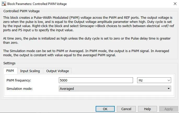
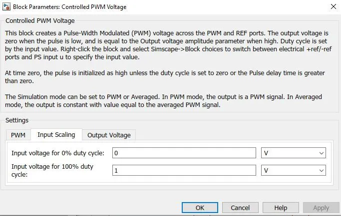
Controlled PWM Voltage parameters -
The parameters are shown below -
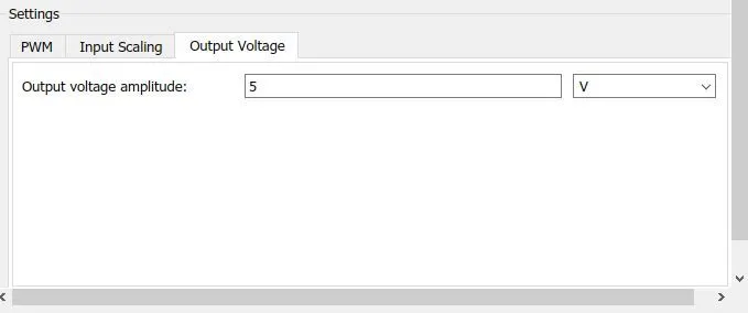
4. Controlled voltage source -
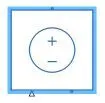
The Controlled Voltage Source block represents an ideal voltage source that is powerful enough to maintain the specified voltage at its output regardless of the current flowing through the source. The output voltage is V = Vs, where Vs is the numerical value presented at the physical signal port.
5. Solver Configuration -
Each physical network represented by a connected Simscape block diagram requires solver settings information for simulation. The Solver Configuration block specifies the solver parameters that your model needs before you can begin the simulation. Each topologically distinct Simscape block diagram requires exactly one Solver Configuration block to be connected to it.
The block has one conserving port. We can add this block anywhere on a physical network circuit by creating a branching point and connecting it to the only port of the Solver Configuration block.
6. Calculation of temperature change -
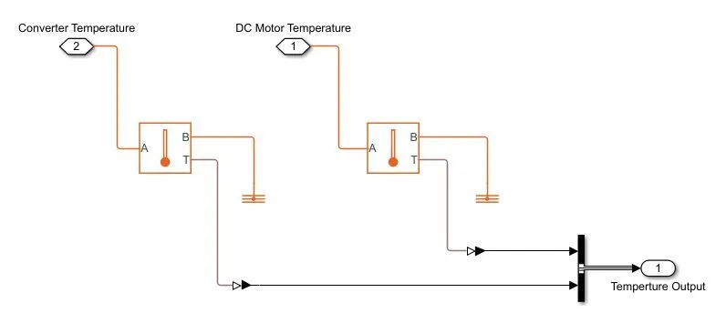
This subsystem is created to observe the temperature changes in the power converter and the DC motor. A temperature sensor is connected to the thermal ports of the converter and the DC motor. The outputs from these sensors are passed through a bus creator which will then be recorded in the scope block.
a. Temperature sensor -
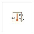
The Temperature Sensor block represents an ideal temperature sensor, that is, a device that determines the temperature differential measured between two points without drawing any heat. Connections A and B are thermal conserving ports that connect to the two points where the temperature is being monitored. Port T is a physical signal port that outputs the temperature differential value.
The block positive direction is from port A to port B. The measured temperature is determined as T = TA – TB.
b. Bus creator -
The Bus Creator block combines a set of input signals into a bus. We can connect any signal type to the input ports, including other buses. We can access signals in a bus by using a Bus selector block.
Elements of a bus must have unique names. By default, each element of the bus inherits the name of the signal connected to the Bus Creator block. If duplicate names are present, the Bus Creator block appends the port number to all input signal names.
BUILDING THE DRIVER CONTROL SYSTEM -
For this, we use a block called Longitudinal Driver.
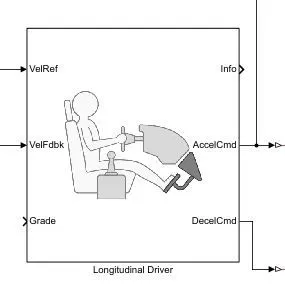
The Longitudinal Driver block implements a longitudinal speed-tracking controller. Based on reference and feedback velocities, the block generates normalized acceleration and braking commands that can vary from 0 through 1. You can use the block to model the dynamic response of a driver or to generate the commands necessary to track a longitudinal drive cycle.
The ports are explained below -
Input ports:
1. VelRef - Input port associated with an input reference velocity of the vehicle.
2. VelFdbk - Input port associated with velocity feedback from the vehicle which helps in smooth control of the system.
3. Grade - Input port associated with the inclination of the surface in degrees.
Output ports:
1. info - Output port associated with a bus signal for acceleration, deceleration, error in velocity, etc.
2. AccelCmd - Output port associated with acceleration commands with reference to the input signal.
3. DecelCmd - Output port associated with deceleration commands with reference to the input drive signal.
Longitudinal Driver parameters -
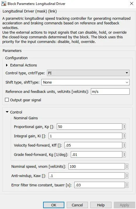
BUILDING THE BATTERY SYSTEM
The battery system is built-in Simulink as shown below.
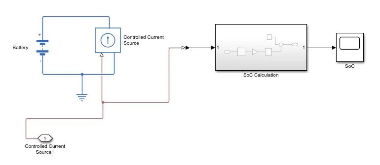
It is a simple circuit connected through a battery and a controlled current source which is in turn connected to the power converter.
Let us look into the blocks used and the SoC calculation subsystem.
1. Battery -
The Battery block represents a simple battery model.
If we select Infinite for the Battery charge capacity parameter, the block models the battery as a series resistor and a constant voltage source. If you select the Battery charge capacity parameter, the block models the battery as a series resistor and a charge-dependent voltage source. In the finite case, the voltage is a function of charge and has the following relationship:
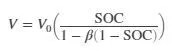
where:
SOC(state-of-charge) is the ratio of current charge to-rated battery capacity.- V0 is the voltage when the battery is fully charged at no load, as defined by the Nominal voltage, Vnom parameter.
- β is a constant that is calculated so that the battery voltage is V1 when the charge is AH1. Specify the voltage V1 and ampere-hour rating AH1 using block parameters. AH1 is the charge when the no-load (open-circuit) voltage is V1, and V1 is less than the nominal voltage.
The equation defines an approximate relationship between voltage and the remaining charge. This approximation replicates the increasing rate of voltage drop at low charge values and ensures that the battery voltage becomes zero when the charge level is zero. The advantage of this model is that it requires few parameters, which are readily available on most datasheets.
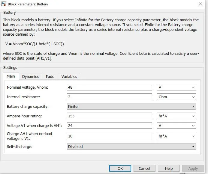
Battery Parameters -
The parameters considered for our model is shown below -
2. Controlled Current source -
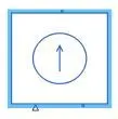
The Controlled Current Source block represents an ideal current source that is powerful enough to maintain the specified current through it regardless of the voltage across the source.
The output current is I = Is, where Is is the numerical value presented at the physical signal port. The positive direction of the current flow is indicated by the arrow.
The block has one physical signal input port and two electrical conserving ports associated with its electrical terminals.
3. Calculation of State of Charge (SoC) -
The state of charge of a battery is calculated as shown below.
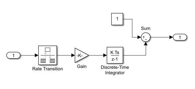
The blocks used in this subsystem are explained below.
1. Rate transition -
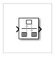
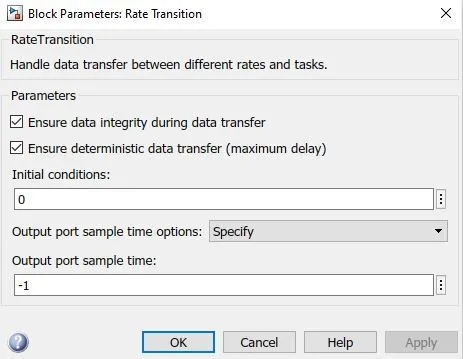
The Rate Transition block transfers data from the output of a block operating at one rate to the input of a block operating at a different rate. Use the block parameters to trade data integrity and deterministic transfer for faster response or lower memory requirements. To learn about data integrity and deterministic data transfer, see Data Transfer Problems (Simulink Coder).
2. Gain Block -
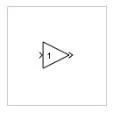
The Gain block multiplies the input by a constant value (gain). The input and the gain can each be a scalar, vector, or matrix.
We can specify the value of gain in the Gain parameter. The Multiplication parameter lets us specify element-wise or matrix multiplication. For matrix multiplication, this parameter also lets us indicate the order of the multiplicands.
Gain is converted from doubles to the data type specified in the block mask offline using round-to-nearest and saturation. The input and gain are then multiplied, and the result is converted to the output data type using the specified rounding and overflow modes.
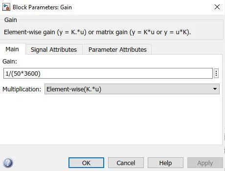
We will be multiplying the input by the value mentioned in the above image.
3. Discrete Block -
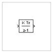
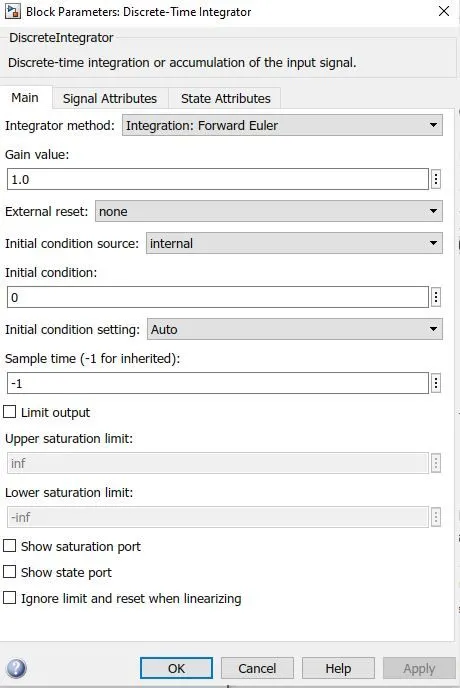
We use the Discrete-Time Integrator block in place of the Integrator block to create a purely discrete model. With the Discrete-Time Integrator block, you can:
- Define initial conditions on the block dialog box or as input to the block
- Define an input gain (K) value
- Output the block state
- Define upper and lower limits on the integral
- Reset the state with an additional reset input
4. SUM block -
The SUM block performs addition or subtraction on its inputs. In this block, the negative terminal will be connected with a discrete-time integrator and the positive terminal with a constant.
BUILDING THE OUTPUT AND INPUT FOR THE MODEL -
The output where we can find the results is shown below.
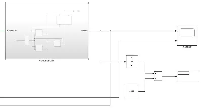
The distance will be calculated using an integrator block. If we integrate the speed, we obtain distance and is then displayed.
Similarly, the input which is given to the driver controller is shown below.
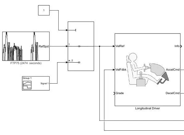
We can see from the above image that a drive cycle input and a signal builder input are given to the longitudinal driver block through a multiport block. Different drive cycles can be given as input to the controller and we can also make our own drive cycle through a signal builder and provide it as an input.
With this, all our subsystems are ready with their respective blocks and parameters. We connect them all and build a complete working model of an electric rickshaw which is shown below.
THE FINAL MODEL AFTER CONNECTING ALL THE SUBSYSTEMS AND BLOCKS -
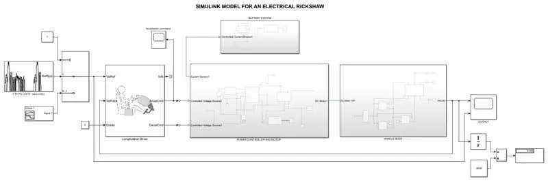
Now that we have our Simulink model of an electric rickshaw, we run it and observe the results.
RESULTS -
1. FTP75 DRIVE CYCLE -
The drive cycle block represents a block that generates a drive cycle for a particular time. It is basically time vs speed data that is similar to that of real-time driving conditions with acceleration and deceleration in an irregular pattern.
By default, the FTP75 drive cycle is selected. Wide-Open throttle conditions can also be selected. Drive cycle data can be taken from spreadsheet data or through a glider block or a signal builder block.
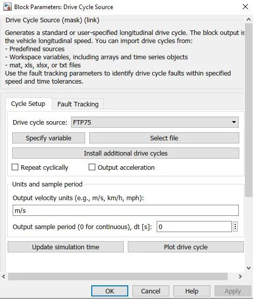
The drive cycle when traced will be as shown below and this will be used as a reference velocity curve.
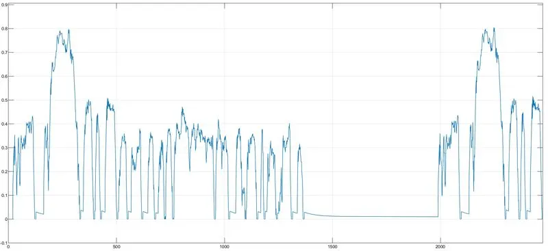
The simulation time will be 2474 seconds.
Distance traveled will be 5.04m/s or approximately 20km.
Actual speed Vs Reference Speed of the vehicle -
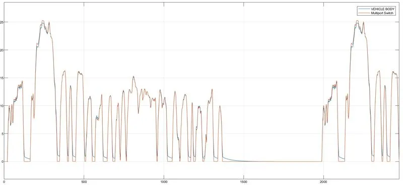
We can see from the above image that the reference velocity of the vehicle (red curve) is almost in line with the actual velocity of the vehicle (blue curve) with a maximum speed of around 25m/s. The small deviation is due to the inertial effect and its control parameters.
State of Charge of the battery -
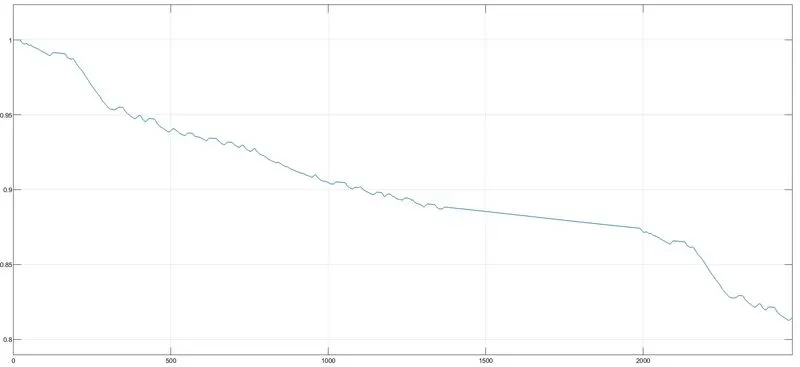
The above image shows the SoC of the battery. For 2474 seconds the battery reaches from 100% to approximately 82%. Almost 20% battery is consumed for the vehicle to travel the distance. Also, we can observe a rise in the SoC curve at some points due to regenerative braking that charges the battery.
The temperature change in converter and motor -
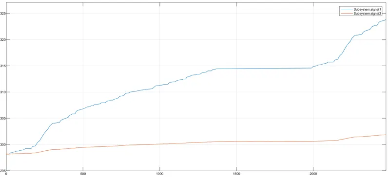
The above image shows the change in temperature of the converter and the DC motor as the vehicle runs. We can observe that the temperature of the DC motor rises continuously and reaches 302 K (29 deg C) and the temperature of the power converter rises to 324 K (51 deg C). As expected the temperature of the components increases as the vehicle runs for a longer period of time. We can also observe that the temperature remains constant when the vehicle is at rest or slowing down.
2. WIDE OPEN THROTTLE CONDITION (WOT) -
The parameters for WOT condition are shown below.
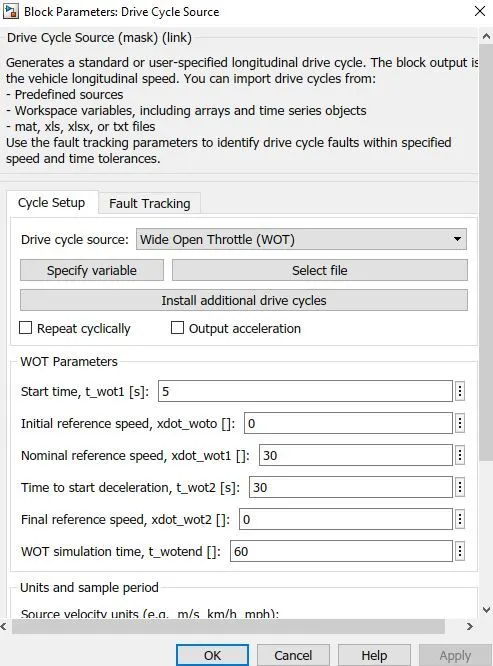
The Simulation time for this condition is 60 seconds.
The plot of the input is shown below.
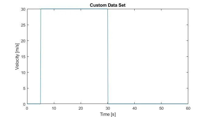
We can see that the acceleration of the vehicle starts at 5 seconds and will be in open throttle condition for 25 seconds in total. Then, at the 30th second, it drops and will be in rest position for the rest of the time. We will input this as a reference speed and compare it with the actual speed of the vehicle in the model.
Acceleration command from the driver controller block-
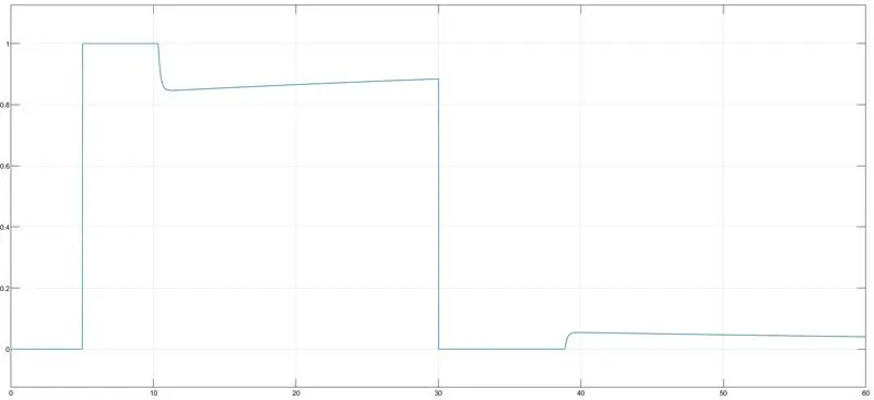
This is the actual driver command which acts as a throttle input. We can see it matches with the input data with a few variations.
Reference speed Vs Actual speed -
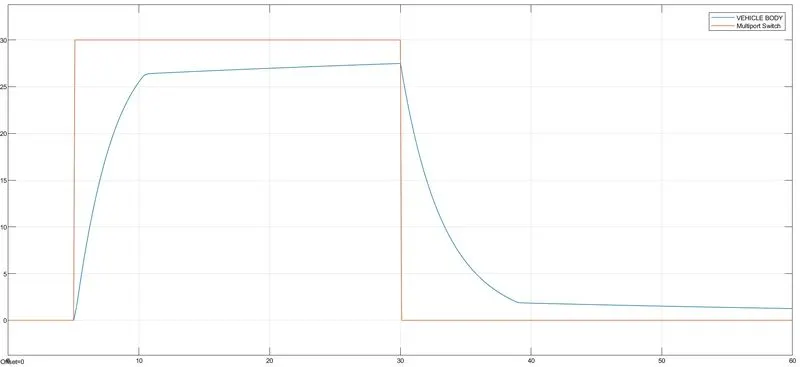
In the WOT condition, we can see the difference between the actual vehicle speed (blue curve) and the reference speed (red curve). In practical conditions, the exact WOT principle is hard to match due to many reasons.
Temperature change in the controller and DC motor-
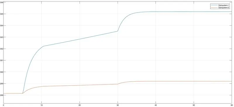
We can see from the above image that the DC motor will reach up to 26 deg C (299 K) and the controller system will reach up to 32 deg C (305 K) in this WOT condition.
State of Charge of the battery -
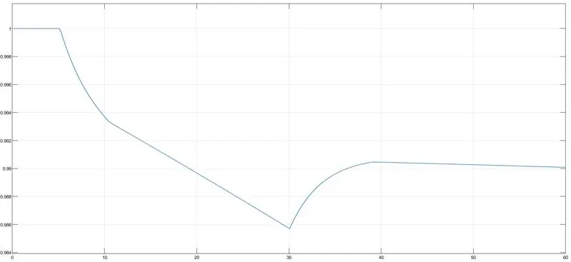
We can observe from the image that, the Soc of the battery will be 99% at the end of the simulation. At the 30th second, we can observe that the battery is at 98.6% charge but due to regenerative braking, we can see a rise in the SoC, and hence it will reach 99%.
3. DRIVE CYCLE THROUGH A SIGNAL BUILDER BLOCK -
We will now build our own driving cycle curve with the use of a signal builder block as shown below.
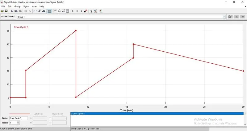
The vehicle will for a total of 30 seconds, it will first accelerate to 20m/s and then will accelerate uniformly to a maximum speed of 50m/s. It will drop to 0 at the 9th second of the simulation time. Then it will rise to a speed of 30m/s and then 40m/s. After this, it will gradually go down to a speed of 20m/s at the 30th second.
The simulation time will be 30 seconds.
Acceleration command from the driver controller block-
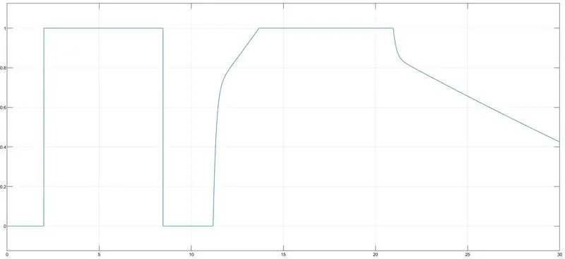
This is the actual driver command which acts as a throttle input. We can see it matches with the input data with a few variations.
Reference speed Vs Actual speed -
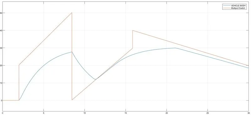
This result is almost similar to the WOT condition. The variations of the actual speed of the vehicle have increased which we can observe in the above image. The reference line is the red curve and the actual speed is the blue curve. To reduce the variations and the differences, we need to tune our parameters in the model.
Temperature change in the controller and DC motor-
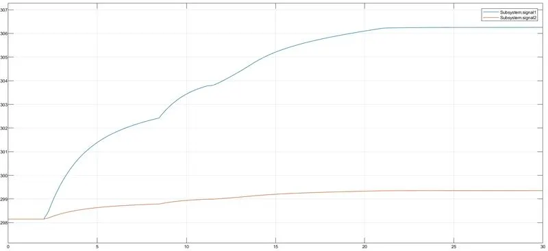
We can see from the above image that the DC motor will reach up to 26 deg C (299 K) and the controller system will reach up to 33 deg C (306 K) for the given driver cycle.
State of Charge of the battery -
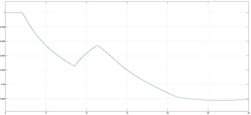
We can observe the variation of the state of charge of the battery during the simulation in the above image. It keeps decreasing to 99.2% and then due to the regenerative braking, it increases to a value of 99.5%. The final SoC of the battery at the end of the simulation is 98.8% as shown in the above image.
CONCLUSION -
As per the motor specification, type of controller, vehicle parameters, and battery used we could see that the reference speed almost matches with the vehicle speed for the drive cycle FTP75. For the WOT condition, a few variations were found in the actual speed of the vehicle. In the third case, the difference between the actual speed and the reference speed is more. Hence, we have to further change the parameters of the system and try simulating to achieve the results.
The parameters that can be changed/improved are stated below -
1. Detailed simulation rather than performing averaged mode simulation
2. Optimization of the battery pack for increased mileage and peak performance
3. Optimization in the vehicle parameters such as vehicle mass, frontal area, drag, tire design, etc.
4. Better motor characteristics or motors such as BLDC motor, which reduces the losses produced from brushes and better efficiency. Hence, better motor power and torque can be achieved.
5. Use of an actual PID controller system rather than the basic PWM signal generator bloc. This enables us to tune the system accordingly and brings down the error.
The Simulink model of the electrical rickshaw is attached below.
The excel sheet containing the list of assumed input data for the Simulink model is attached below.