Final Project: Electric Rickshaw modelling

Aim: To develop a detailed MATLAB model of a three-wheeler electric rickshaw

Objectives:

Using permanent brushed type motor which drives the rear wheels.

To create a custom derive cycle using an excel sheet

Simulate the required model for three standard derive cycle

Energy consumption, temperature rise of motor and controller

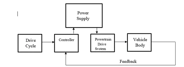
Block Diagram of a typical electric rickshaw:

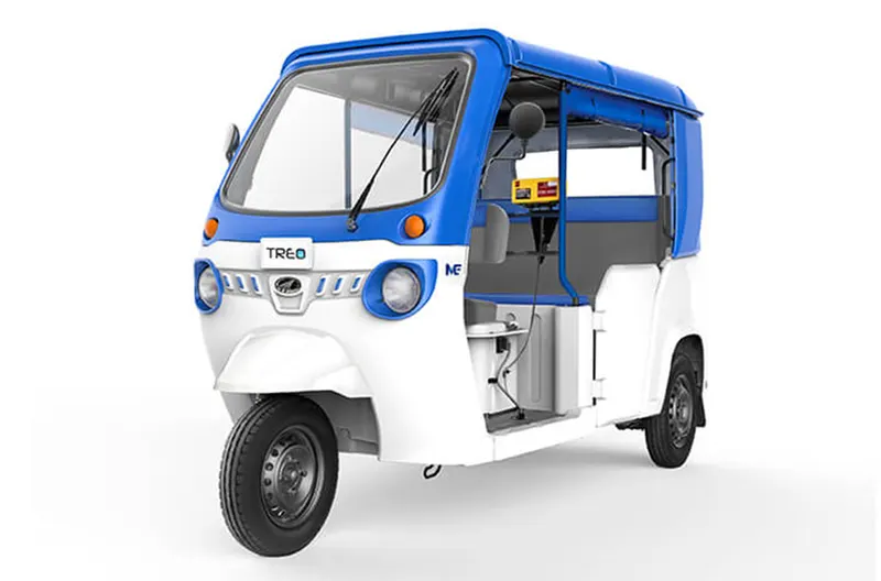
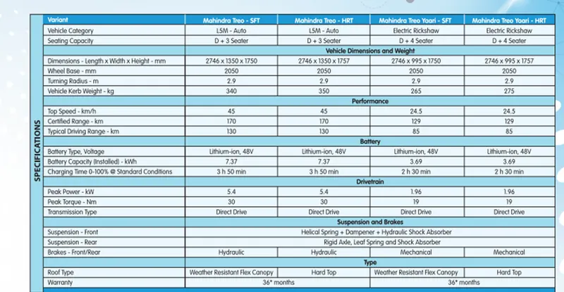
Mahindra Treo is taken as reference for the modeling purpose:

Simulink Model of three-wheeler E- Rickshaw:

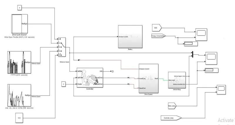
Major Components:

(I)Drive Cycle: The input or reference speed is called drive cycle. Shown below are three standard drive cycle

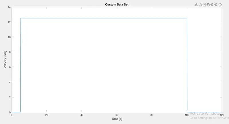
(1) Wide open throttle (WOT): In this type of derive cycle, full throttle is given for the particular duration of time

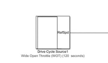
The above block generates a standard or user-specified longitudinal drive cycle. The block output is the vehicle's longitudinal speed.

Plot of WOT drive cycle:

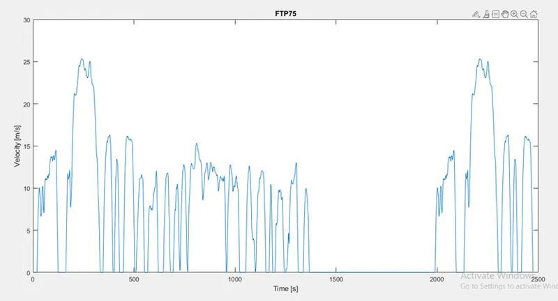
(2) FTP75: This drive cycle shows the urban driving pattern for a duration of 2475 sec

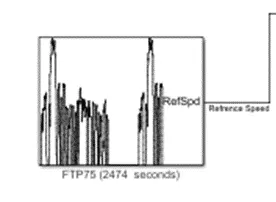
plot of FTP75 drive cycle:

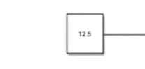
(3) Constant Speed Drive cycle: For calculating the energy consumption, rise in temperature of the motor controller for a constant speed of 45kmph or 12.5m/s for a distance of 100km

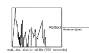
(4) Custom drive cycle: A custom drive cycle is prepared using excel datasheet for a duration of seconds

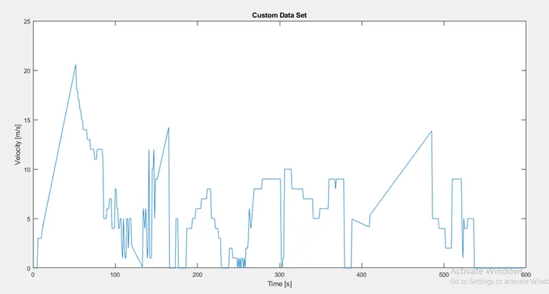
Plot of custom drive cycle:

• Multiport Switch:

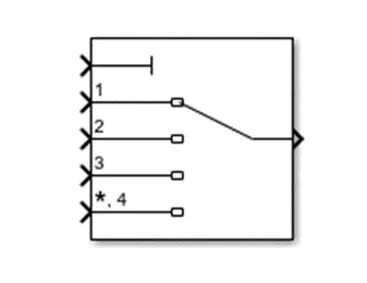
To select a particular drive cycle from the available multiport switch is used. The selection can be made with the help of port 1.

(II) Controller: The speed of the vehicle is being measured and fed to the controller. The controller compares the reference speed with the actual speed and generates actuating signal according to the error. In this model, the control of speed is being achieved by giving acceleration and deceleration commands to a controlled PWM voltage source which manipulates the voltage fed to the DC motor through an H bridge. In actual conditions, the control is achieved by controlling the power supplied by the battery.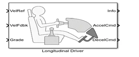

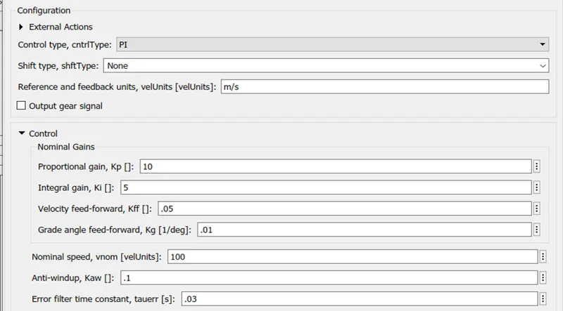
• Configuration of the controller and control parameter specifications is shown below:

(III) Drive/powertrain System:

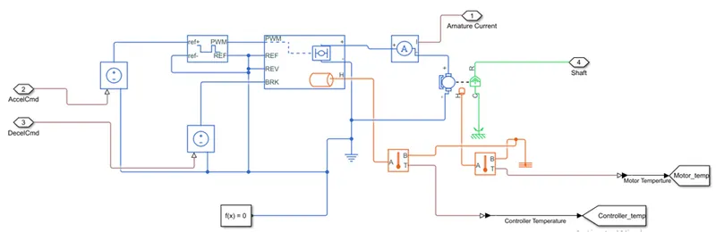
The powertrain in this model consists of the controller voltage source, controlled PWM voltage, H-bridge, current sensor, DC motor, and temperature sensor:

Components:

Controlled Voltage Source (CVS):

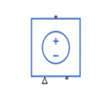
CVS is used to give control commands (acceleration and deceleration) command to PWM voltage block

Controlled PWM voltage:

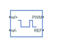
Pulse width modulated (PWM) voltage across PWM and REF port is produced by this block to control the voltage fed to the armature of DC motor by the H-bridge.

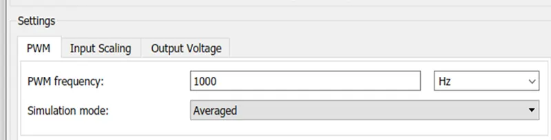
In the simulation averaged mode is used and PWM frequency is taken as 1000Hz

H-bridge: This block is driven by controlled PWM voltage in PWM and averaged mode. Averaged mode is used for the simulation to reduce the simulation time taken.

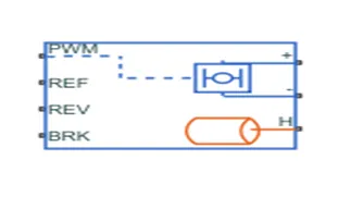
Port ‘H’ is the thermal port that can be used to observe the temperature of motor. This port can be made visible by right-clicking on the block and from the block choices in simspcape choose show thermal port.

The H-bridge is configured to following settings

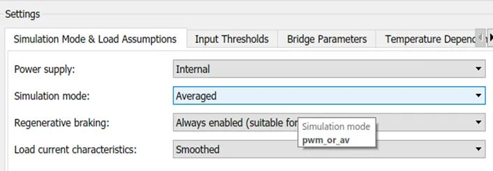
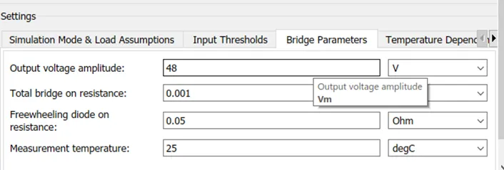
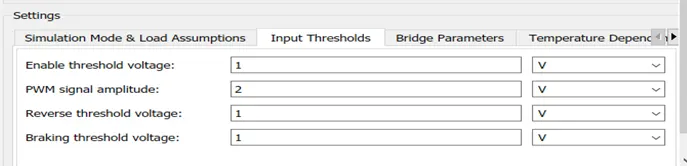
As the DC motor has a 48 voltage rating so the output of the H-bridge is taken as 48V

DC-motor:

The block shown below represents a permanent magnet 48V, 5.4kW DC motor

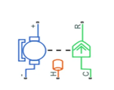
When a positive current flows from the electrical + to - ports, a positive torque acts from the mechanical C to R ports

H is the thermal port which is hidden by default and can be made visible by selecting show thermal port from simscape block.

Specifications:

Armature inductance: 12*10^-6 nH

No-load speed: 1800 rpm

Rated speed (at rated load): 1710 rpm

Rotor inertia: 0.01g*cm^2

Initial temperature: degC

Thermal mass: 20 kJ/K

Temperature sensor:

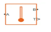
In a thermal network, this block measures temperature. The sensor does not have any heat flow. The temperature difference across the sensor is reported by the physical signal port T. When the temperature at port A is higher than the temperature at port B, the measurement is positive.

Current Sensor: The current flowing through the armature is measured and fed to a current-controlled source, which mimics the operation of battery discharging

(IV) Battery system:

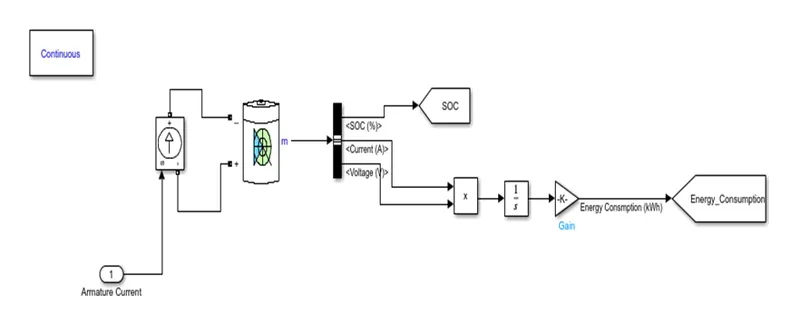
In this simulation model, actual voltage is not fed to the motor, instead, the armature current is used to mimic the battery state, with this SOC and energy consumption can be calculated

Specification:

Type: lithium-ion

Nominal voltage: 48V

Rated capacity: 120 Ah

(V) Vehicle body: The most weight is essentially contributed by the vehicle body itself in an electric vehicle. The vehicle body encloses all the other components. The body weight has to be optimized to have maximum efficiency. E rickshaw is comparatively lightweight

In MATLAB the vehicle body be represented by blocks as shown below:

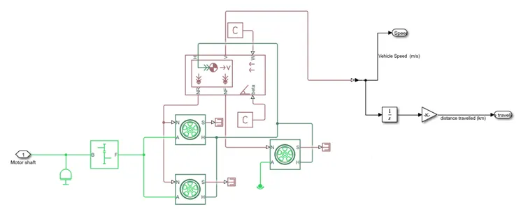
Output of motor shaft is connected to the axel and wheel through a simple gear.

Components:

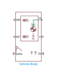
Above block represents a two-axle vehicle body in longitudinal motion.

Ports:

H: Mechanical translation conserving port, tires should be connected to H

V, NR, NF: Physical signal output ports for vehicle velocity and front and rear normal wheel forces, respectively.

W, beta: Physical signal input ports corresponding to headwind speed and road inclination angle, respectively.

Specifications: Vehicle specifications are taken from the Mahindra Treo model, shown below:

Mass of Vehicle: 340kg

Frontal area: 1.35 m^2

Drag coefficient: 0.5

Air density: 1.18 kg/m^3

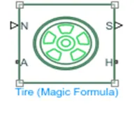
• Tires (Magic formula):

• Ports:

  A: Mechanical rotational conserving port for the wheel axle.

  N: Physical signal input port that applies the normal force acting on the tire.

  S: Physical signal output port that reports the tire slip.

  Specifications:

  Rated vertical load: 3000N

  Peak longitudinal force at rated load: 3500N

  Slip at peak force at rated load (percent): 10

  Rolling radius: 0.3m

• Simple gear:

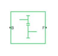
Connections B (base) and F (follower) are mechanical rotational conserving ports

Follower (F) to base (B) teeth ratio (NF/NB): 2

The output shaft rotates in the same direction as the input shaft.

• Inertia:

This block represents an ideal mechanical rotational inertia.

Results:

(1): Wide open throttle input: run-time-120sec

(a) Speed and distance

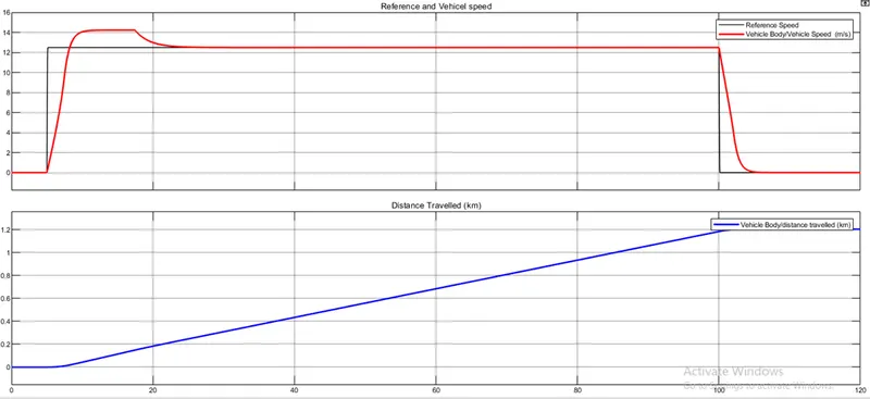
Vehicle tracks reference speed with some delay and overshot

Distance traveled: 1.204km

(b) SOC(%) and Energy consumption

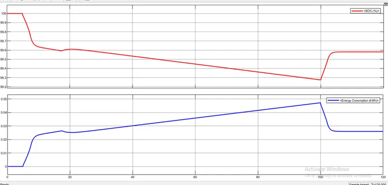
During retardation, regenerative braking takes place, therefore the SOC (%) starts increasing after 100sec

At the end of the drive cycle:

SOC(%) ~99.59

Energy consumed~ 0.02599 kWh

(c) Motor and Controller temperature

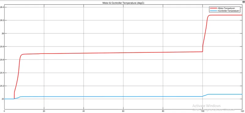
Initially at 5sec, when there is sharp increase in the reference and thus motor speed, so temperature of motor rises significantly. For Constant speed duration the motor and controller temperature increases very gradually and for the duration when the motor stops, the controller and motor temperature remains constant.

At the end of drive cycle

Motor temp~26.3­­^o

Controller temp~25.1^o

(2) FTP75 dive cycle input: Run-time 2474sec:

(a) Speed and distance

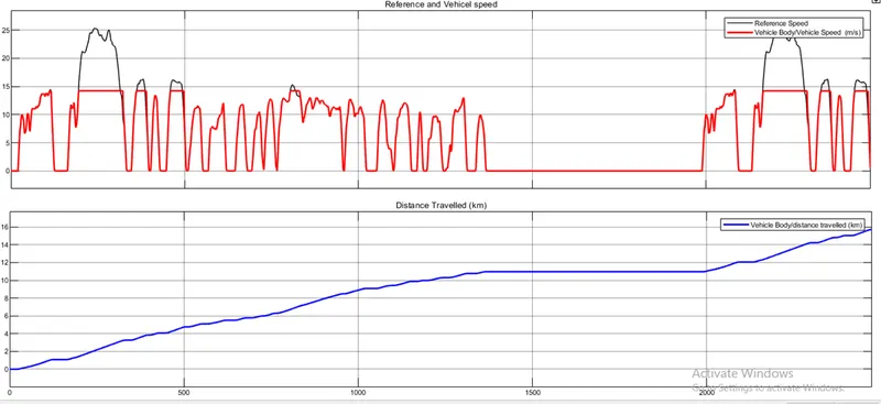
The vehicle fairly tracks the reference speed, but after about 150sec the vehicle saturates at about 15m/s, this is due the motor maximum speed is limited for the particular power rating.

Distance travelled: 15.73km

(b) SOC (%) and Energy consumption:

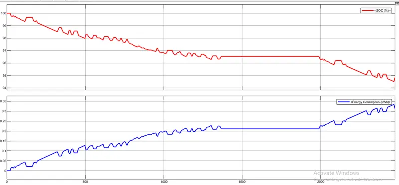
At the end of the drive cycle

SOC (%) ~ 94.5

Energy Consumption: 0.1323kWh

(c) Motor and Controller temperature

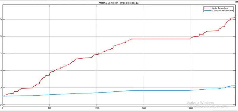
At the end of the drive cycle

Motor temp~34.5­­^o

Controller temp~26.3^o

(3) For custom drive cycle input: run-time 596 sec

(a) Speed and distance

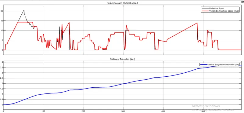
For speed less than the rated speed, the vehicle tracks the custom duty cycle too, it shows that the controller is robust and gives satisfactory results for every drive cycle.

(b) SOC (%) and Energy consumption:

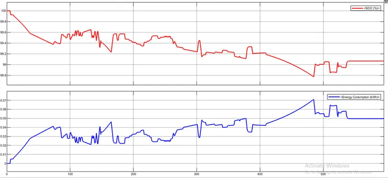
At the end of the drive cycle

SOC (%) ~ 99

Energy Consumption: 0.05kWh

(c) Motor and Controller temperature

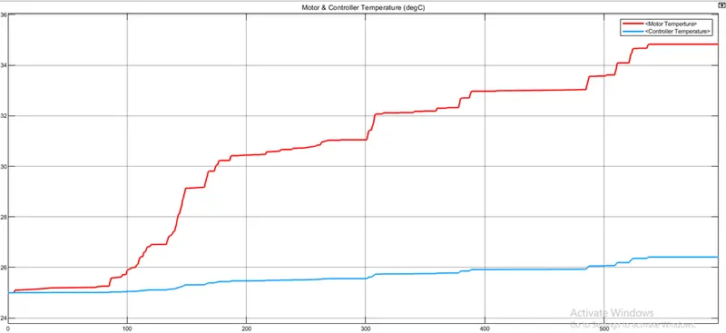
Motor temp~35^o

Controller temp~26^o

(4) Constant Speed of 45kmph or 12.5m/s: Run time 8000 sec

(a) Speed and distance:

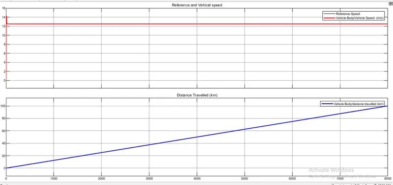
As the desired reference speed is less than the rated speed so the vehicle successfully tracks the desired speed

Distance travelled: 100km

(b) SOC (%) and Energy consumption:

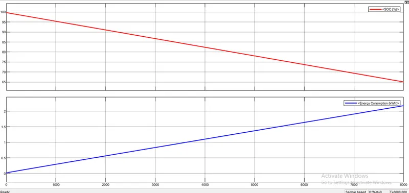
At the end of driving cycle

SOC (%) ~ 65

Energy Consumption: 2.15 kWh

(c) Motor and Controller temperature

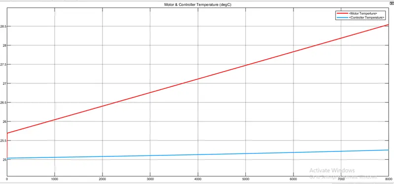
Motor temp~28.5^o

Controller temp~25.3^o

^{Conclusion: The Aim of the project is successfully achieved and the model showed good performance and the results indicate the model is close enough to the actual system}

^{References: https://www.mahindraelectric.com/pdfs/mahindra-treo-eBrochure.pdf}

^{https://trucks.cardekho.com/en/trucks/mahindra/e-alfa-mini/specifications}

^MTALAB/elp