Final Project: Electric Rickshaw modelling

Electric Rickshaw modelling

AIM

• Create a detailed MATLAB model of an electric rickshaw (three-wheel passenger vehicle)

OBJECTIVES

• Rear wheels driven by PM brushed type motor
• Assume efficiency points of motor controller and motor
• Make an excel sheet of all input and assumed data
• For any three standard driving cycles show energy consumption, temperature rise of motor and controller for 100 km constant speed driving at 45 kmph.

ABSTRACT

• Global efforts towards minimizing greenhouse gas emissions are required to reduce the environmental issues caused by conventional combustion engine vehicles. Alternate clean and green modes of transportation such as electric vehicles are required in place of conventional vehicles. As a cheaper version of electric vehicle, electric rickshaws (popularly known as E-rickshaws or tuk-tuks) are most popular in India. This work deals with the modelling of popular e-rickshaws in MATLAB/Simulink. Software simulations are much helpful for quickly analysing the distinct features of the electric vehicle, such as aerodynamic design, battery energy density, motor output, curb weight, etc and to visualize the effects on its performance due to variation in various parameters. Therefore, simulations were performed with Simulink model of e-rickshaw with battery packs. The simulation results favour the possibility of implementing simultaneous battery packs at a reasonable cost price

THEORY

Electric rickshaw

• Electric rickshaws (also known as e-rickshaws or tuk-tuks) have been becoming more popular in some cities since 2008 as an alternative to auto rickshaws and pulled rickshaws because of their low fuel cost, and less human effort compared to pulled rickshaws. They are being widely accepted as an alternative to petrol/diesel/CNG auto rickshaws. They are three-wheelers powered by an electric motor ranging from 650 to 1400 Watts. They are mostly manufactured in India and China. Battery-run rickshaws could be a low-emitter complementary transport for the low-income people, who suffer most from a lack of transport facility, if introduced in a systematic manner according to experts.

E-rickshaw Market in India

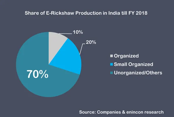
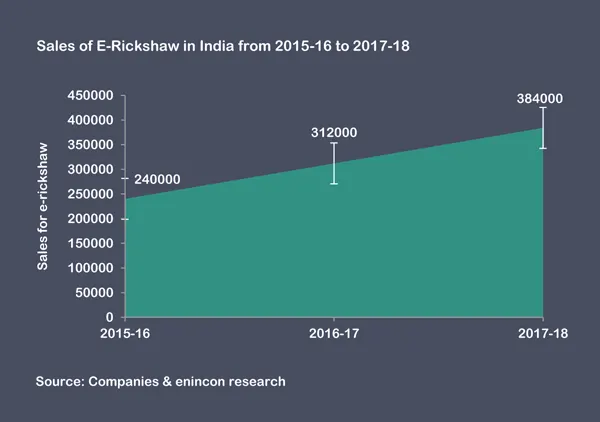
• E-Rickshaw's have now transitioned from being a market entrant in the automobile segment of the country to evolve as a leading short-distance transport solution.
• This segment has gained spurt in last three years and the growth has been phenomenal. Although, this segment is dominated by a host of unorganized players the established names have also identified the growth beacon and are expected to foray into the segment.
• The share of production for e-rickshaws for now is indicated.
• Though introduction in India did happen on the lines of China in the late 2010s but was very sporadic and was not spread across. It was the drive to have greener transport industry especially in tier-2 & tier-3 cities the e-rickshaw market is vastly gaining base and is likely to grip on further in coming years with the advent of established players in the segment as well. The actual sales value for e-rickshaws in India is depicted in Exhibit.

Design and construction (Benchmarking)

• These rickshaws have a M.S(Mild Steel) tubular Chassis, consisting of three wheels with a differential mechanism at the rear wheels. The motor is brushless DC motor manufactured mostly in India and China. The electrical system used in Indian version is 48V and Bangladesh is 60V. The body design from most popular Chinese version is of very thin iron or aluminum sheets. Vehicles made in fibre [clarification needed] are also popular because of their strength and durability, resulting in low maintenance, especially in India. Body design is varied from load carriers, passenger vehicles with no roof, to full body with windshield for driver's comfort. It consists of a controller unit. They are sold on the basis of voltage supplied and current output, also the number of MOSFET (metal oxide field effect transistors) used. The battery used is mostly lead acid battery with life of 6–12 months. Deep cycle batteries designed for electric vehicles are rarely used. Weight of the electric car has also been a recurring design difficulty in them.

DESIGN AND DEVELOPMENT

E - Rickshaw Powertrain

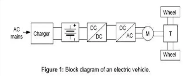
• An EV’s powertrain is responsible for taking energy stored in the vehicle’s battery system and supplying it to the motors.
• Power flow is from the battery to the power converter and to the PM DC motor and to the differentials and finally to the wheels.

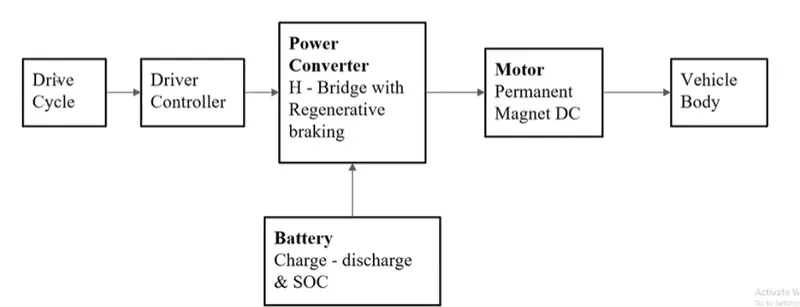
• The main blocks of the electric rickshaw model are the battery, the drive cycle, the controller, the DC motor, and the vehicle body & transmission system.
• Drive cycle is the input data, The Drive-cycle basically is the representative of the road. The main purpose is to gain the required speed through the driver input, calculate the temperature of the motor and controller, calculate the charge levels (soc) and the distance travelled by the vehicle. There is also a Soc block that measures the charge level of a battery, and the distance is calculated according to the speed and time parameters of all three drive cycles.

Power requirements

• Load power requirement is calculated based on the drive cycle and vehicle dynamics. Energy source sizing is carried out based on this power requirement.

Drive Cycle

• The Drive Cycle Source block generates a standard or user-specified longitudinal drive cycle. The block output is the specified vehicle longitudinal speed. The load power requirement was calculated for the driving cycle. Battery was sized based on this power requirements. Modelling of vehicle dynamics is explained in detail in the following sections.

Vehicle dynamics

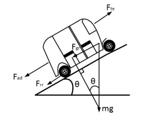
• The forces acting on a vehicle needs to be understood for an effective modelling of vehicle dynamics. The forces acting on an auto-rickshaw while hill climbing is shown in Figure. The tractive force generated by the electric motor of the vehicle has to experience and overcome these forces namely (a) Rolling resistance force (b) Aerodynamic drag (c) Grade resistance force and (d) Acceleration force
• The major forces acting on an E-rickshaw and their expressions are shown in Table:

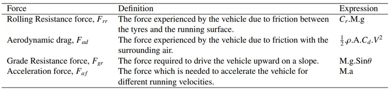
• Here, M is the mass of the vehicle in kg, g is the gravitational constant, i.e., 9.81 m/s^2, Cr is the coefficient of rolling resistance, ρ is the air density in kg/m^3, A is the frontal area of vehicle in m^2, Cd is the drag coefficient, v is the velocity of the vehicle in m/s, θ is the clockwise angle made by the slope of the road with the horizontal plain and a is the acceleration of the vehicle in m/s^2.
• The total tractive force is the force required to propel the vehicle forward by overcoming all the above-mentioned forces acting on the vehicle. Neglecting all other forces acting directly or indirectly on the vehicle, the total tractive force can be obtained from the Eq,
  `F_(te) = F_(rr )+ F_(ad) + F_(gr) + F_(af)`

E-rickshaw System Architecture

• The sizing of every components like energy source,electric motor, power electronic converters etc., of an E-rickshaw depends on the vehicle parameters and driving patterns. The total tractive force required by the vehicle for propulsion was calculated using Eq 1.

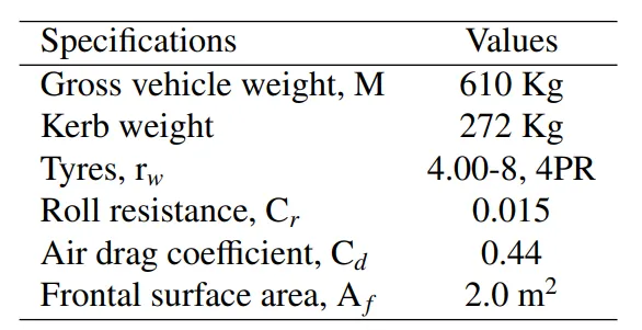
• System parameters like mass of the vehicle, frontal area etc., is available from Table 1. Vehicle velocity and acceleration is obtained from drive cycle data. Required load power is calculated as the product of total tractive force and velocity. The energy flow in a conventional electric-rickshaw is as shown in Figure 3. The vehicle dynamics of an auto-rickshaw is modelled in MATLAB-Simulink environment.

SIMULINK MODEL

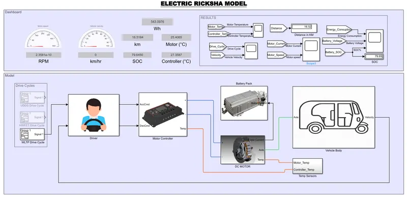
• The Simulink model represents electric rickshaw simulation. We configured the systems into sub-systems so that each subsystem would have the required functionality and we'll get a better understanding of the model.
• The dashboard will indicate the speed of the vehicle, the distance covered by the vehicle, the motor RPM and the battery SOC level.
• The driver subsystem takes input from the drive cycle data and converts it into acceleration and deceleration commands.
• The drive cycles used in this model are UDDS, HWFET, and user-defined drive cycle speed data in m/s.
• The motor controller controls the DC motor using the acceleration and deceleration commands. We used controlled PWM block and H-bridge blocks to obtain the required control of the DC motor.
• The motor controller subsystem is connected to the motor subsystem, where the DC motor is powered and the motor current is passed with the battery subsystem and the soc level and power consumption values are calculated. The rotating part of the motor that rotates the axle is connected to the vehicle plant.
• In the vehicle body, Rotation on the axle is converted into vehicle motion, and in this block the vehicle dynamics forces of the vehicle are considered.
• The final vehicle speed is passed to the driver block as feedback for better control of the vehicle to operate on the required drive cycle.
• Now, each subsystem can be discussed in detail.

VEHICLE BODY

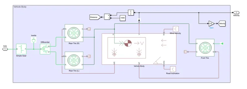
• In Vehicle body we can see Tires, Chassis, Differentials and gear box. we use friction parameterised tire blocks, vehicle body block, differential block and simple gear block to build the vehicle body block.
• Here we add vehicle body from Simscape library which it chases of vehicle. Vehicle body is having six ports. H means Hub, V means actual speed of vehicles. W means wind velocity, delta means inclination offroad. Enough means normal force for front wheel NR means normal posts for rear-view double click on block to change block parameter.
• Connect N to NR of rear wheels and H to H of wheels. Now add differential from Simscape Library. With the help of differential, inertia and loss from gear meshing and viscous bearing friction can be optionally included.
• Then add simple gear. We are going to connect the S terminal of the gear to the D terminal of the differential. Also connect differential S1 & S2 to the wheel axle. To get positive velocity, change the parameter from the gear block. With all these connections we make our vehicle body subsystem. From this subsystem we are going to check the actual speed of the vehicles. Now connect the scope and display to port V of the vehicle body. Now we can measure the actual speed and distance of the vehicle.

• All block parameters are customized according to our model concerns.

Vehicle Body,

• Mass = 610 Kg
• Frontal Area = 2 m^2
• Drag coefficient = 0.44
• Road Inclination = 0
• Wind velocity = 0

Tires,

• Rolling Resistance = 0.015

Simple gear,

• Gear Ratio = 4
• Differential Ratio = 4

DC MOTOR

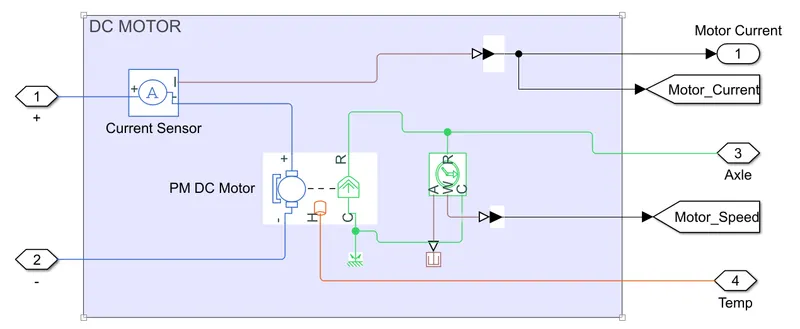
• Add DC motor from Simscape library. To measure current to the motor, current sensor is added. Connect the terminals of the DC motor to the Motor controller. Connect the R terminal of motor to the gear box. C would be connected to the mechanical rotational reference.
• For measuring Rotational speed of the motor, ideal rotational motion sensor is connected to the DC motor.
• By changing Motor parameters we can examine how actual speed is matching the reference speed.

Motor parameters,

• Field type: Permanent Magnet
• Model parameterization: By rated load and speed
• No-load speed: 14000 rpm
• Rated speed (at rated load): 12000 rpm
• Mechanical power: 50KW
• Rated DC supply voltage: 50V
• Thermal mass: 10000 J/K
• Initial Temperature: 25 DegC

• If the rated speed is less, we'll get more difference between actual speed and reference speed. so, if we get more difference between actual speed and reference speed then we can reduce this difference by increasing the rated speed or by decreasing the vehicle body weight.

MOTOR CONTROLLER

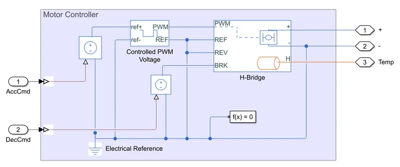
• An H bridge converter was added to control the DC motor. Controlled PWM voltage was added to control PWM input. Now with the help of H-bridge we can perform acceleration, braking and reverse mechanisms.
• The H Bridge requires power supply to operate, and the H Bridge power supply can be applied internally or externally.

H Bridge block parameters,

• Simulation mode: Averaged (will reduce simulation time)
• Output voltage amplitude: 50V
• Enable threshold voltage: 0.0001V
• PWM signal amplitude: 1V
• Reverse threshold voltage: 0.0001V
• Braking threshold voltage: 0.0001V
• Thermal mass: 100000 J/K

Controlled PWM Voltage block parameters,

• Simulation mode: Averaged
• PWM frequency: 5000Hz
• Input Scaling: 0 - 1 V
• Output Voltage Amplitude: 1V

• PWM block will get input from the driver, and driver would providing inputs in terms of 0 or 1. so, we have chosen 0 and 1 as a low value and high value respectively.
• Acceleration and deceleration commands from the driver blocks, a controlled voltage source blocks connected between the reference port and the brake ports of the PWM source block and the H-bridge block.
• All the electric connections would be grounded, and a solver configuration is connected to the ground.

Temperature Sensors

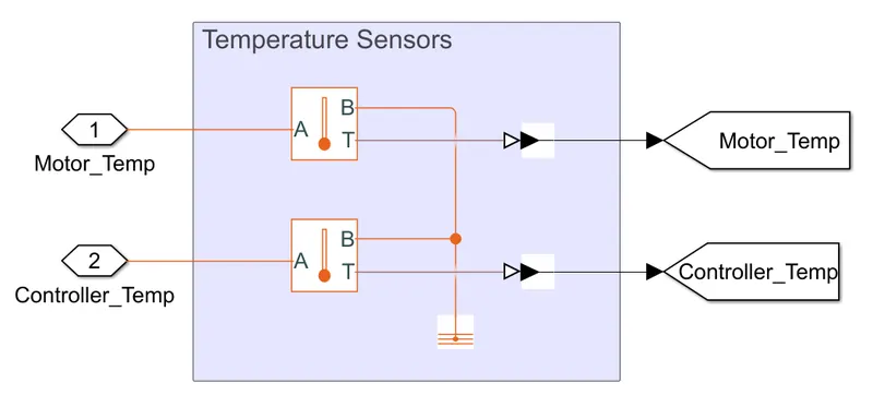
• Temperature outputs from the thermal ports of the motor and motor controller are measured using a temperature sensor block attached to the thermal network, with one port connected to the motor and one to the controller's thermal port, and the other port with thermal reference where the temperature is equal to absolute zero.

BATTERY MODEL

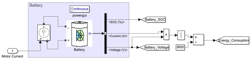
• Battery model is needed to estimate the SOC level and energy consumption of the vehicle model. we used Specialised Power systems Battery model which will give direct SOC estimation, Battery current and voltage.

Battery parameters,

• Battery type: Lithium Ion
• Nominal voltage: 50V
• Rated Capacity: 50Ah
• initial SOC: 100

• Output of the battery is connected with bus selector, and selected all the elements and connected with scope to view the results. Energy consumption can be determined by multiplying Battery voltage and current and integrating it and divide it by 3600.
• Battery terminals are connected with controlled current source block from the power systems fundamental blocks. The motor current is the controlled current to the battery. It represents the current which will flow from battery to motor while accelerating and motor to battery when braking.
• Add power gui block.

DRIVER

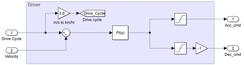
• Here we provide reference signals as standard drive cycles using the Signal Builder block. We connect the actual speed of the vehicle as feedback. A PID block is used to control the driver block, and the driver outputs are acceleration and deceleration commands.
• Using signal builder block standard drive cycles are created, here the velocity values are providing in the unit m/s. so to convert m/s to km/hr we need to multiply the value with 3.6.

• Scopes are used to observe the behaviour of our model and to obtain results. we can observe Drive cycle and actual speed, Distance covered, motor current and motor speed, Motor temperature and Controller temperature, Battery current, battery voltage, Energy consumption and SOC level.

RESULTS

1. Drive Cycle = UDDS (Urban Dynamometer Driving Schedule) (Run Time = 1470sec)

• The cycle simulates a urban route of 12.07 km with frequent stops.
• The maximum speed is 91.25 km/h
• The average speed is 31.5 km/h.

Dashboard

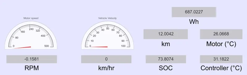
• Distance travelled = 12km
• Battery SOC = 73.8%
• Motor temperature = 26°C (initially 25°C)
• Controller temperature = 31°C (initially 25°C)
• Energy consumption = 687.02 Wh

Actual Speed & Reference Speed

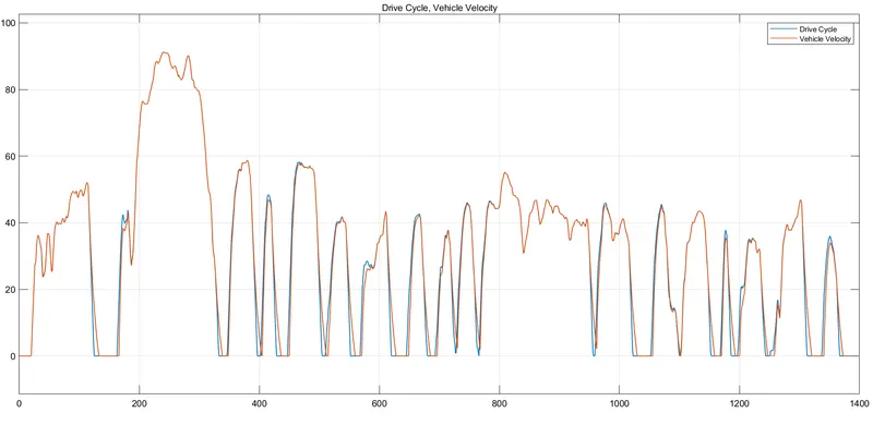
• Actual speed is trying to follow the reference speed, we achieved an average speed of 31.54 kmph.
• The difference between the actual vehicle speed and the reference speed is very small. The vehicle's high-speed ranges completely overlap, while at the slower speeds response needs to be improved, a slight lag is observed.

Motor Current, Motor Speed, Motor & Motor Controller Temperatures

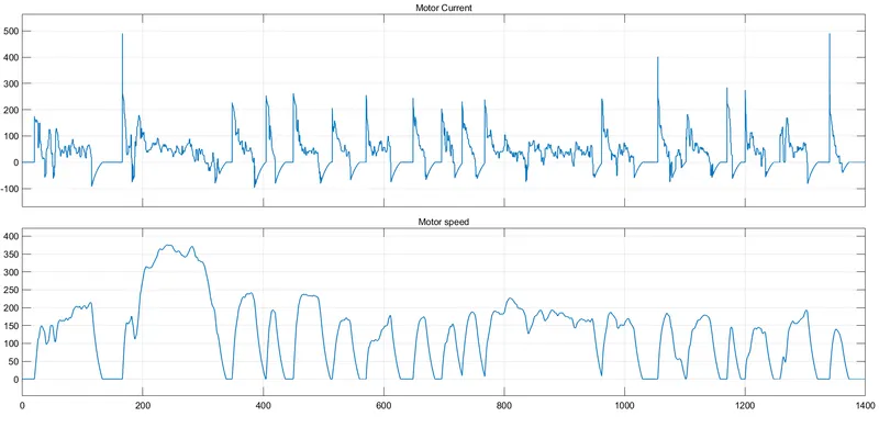
• Motor positive current value indicating the current flowing from battery to the motor and the negative current indicates the regenerative current flows from motor to battery which charges the battery while braking.
• The motor speed is controlled according to the required reference speed

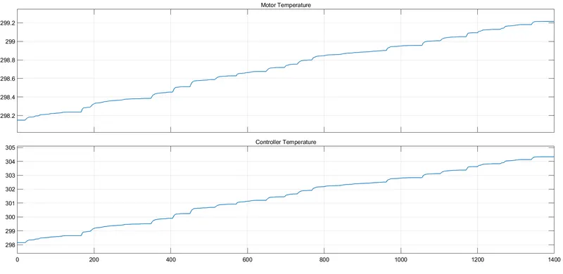
• The motor temperature rises from the initial temperature of 25°C to 26°C. At the same time, the temperature of the motor controller increased from 25°C to 31°C.

Battery Current, Battery Voltage & Battery SOC

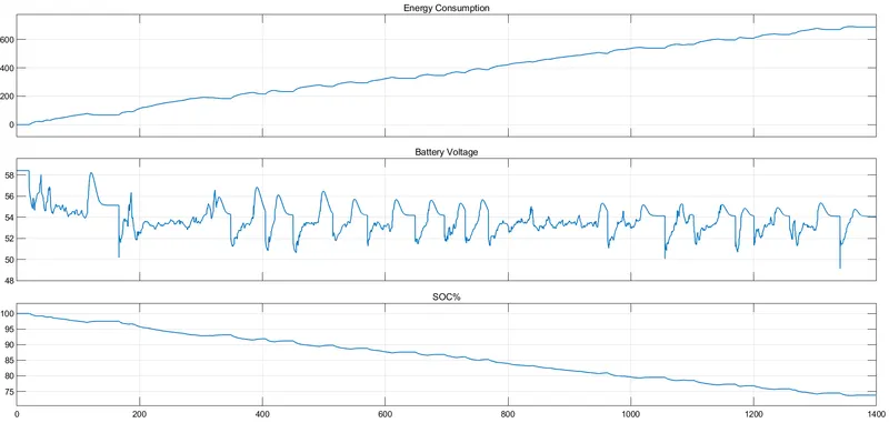
• 687.02Wh of energy is consumed, Battery SOC drops to 73.8%. Battery voltage fluctuates according to motor demand.

2. Drive Cycle = HWFET (Highway Fuel Economy Cycle) (Run Time = 800sec)

• The cycle simulates a Highway route of 16.45 km
• Average Speed is 77.7 km/h

Dashboard

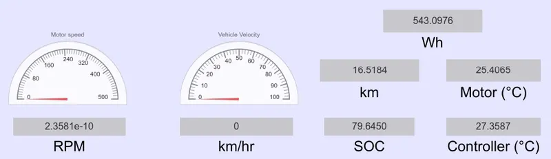
• Distance travelled = 16.51km
• Battery SOC = 79.64%
• Motor temperature = 25.40°C (initially 25°C)
• Controller temperature = 27.35°C (initially 25°C)
• Energy consumption =543.09 Wh

Actual Speed & Reference Speed

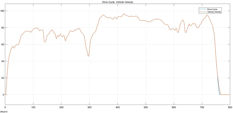
• Actual speed overlaps the reference speed, we achieved an average speed of 77.73 kmph.

Motor Current, Motor Speed, Motor & Motor Controller Temperatures

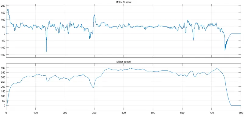
• Motor positive current value indicating the current flowing from battery to the motor and the negative current indicates the regenerative current flows from motor to battery which charges the battery while braking.
• The motor speed is controlled according to the required reference speed.

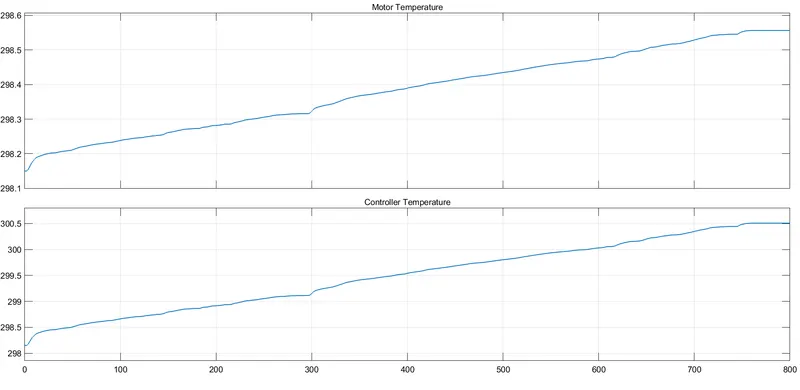
• Since the drive cycle does not have frequent stops, the controller has less work to do and the motor has to rotate without interruption, which reduces the temperature rise during the operation of the motor and the Motor controller.
• The motor temperature rises from the initial temperature of 25°C to 25.4°C. At the same time, the temperature of the motor controller increased from 25°C to 27.31°C.

Battery Current, Battery Voltage & Battery SOC

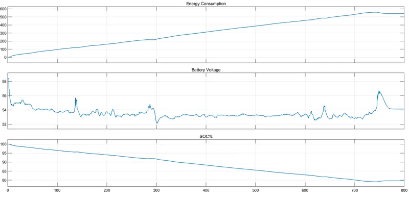
• Energy consumption is 543.09Wh, 16.1km distance covered. Battery SOC drops to 79.65%.
• Battery voltage fluctuates according to motor demand. Less fluctuations than in USSD drive cycle.

3. Drive Cycle = WLTP (Worldwide Harmonised Light Vehicles Test Procedure) (Run Time = 1810sec)

• The cycle simulates a urban route of 23.25 km.
• The maximum speed is 131.3 km/h.
• The average speed is 46.5 km/h.

Dashboard

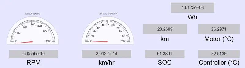
• Distance travelled = 23.26km
• Battery SOC = 61.38%
• Motor temperature = 26.3°C (initially 25°C)
• Controller temperature = 32.5°C (initially 25°C)
• Energy consumption =1.01 KWh

Actual Speed & Reference Speed

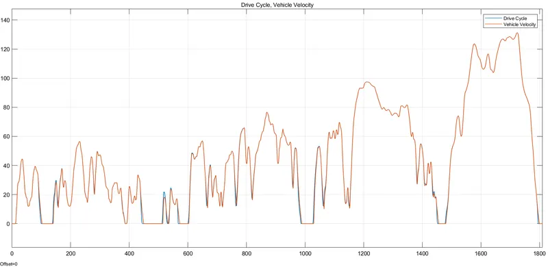
• Actual speed is trying to follow the reference speed. Actual speed almost overlaps the reference speed, we achieved an average speed of 46.3 kmph.
• The difference between the actual vehicle speed and the reference speed is very small. The vehicle's high-speed ranges completely overlap, while at the slower speeds response needs to be improved, a slight lag is observed.

Motor Current, Motor Speed, Motor & Motor Controller Temperatures

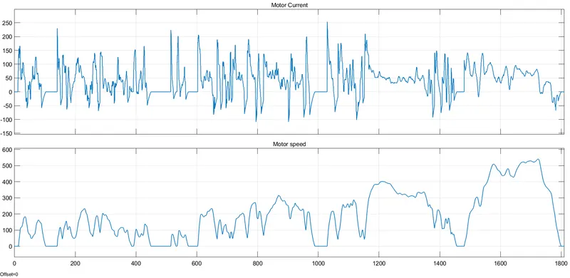
• Motor positive current value indicating the current flowing from battery to the motor and the negative current indicates the regenerative current flows from motor to battery which charges the battery while braking.
• The motor speed is controlled according to the required reference speed.

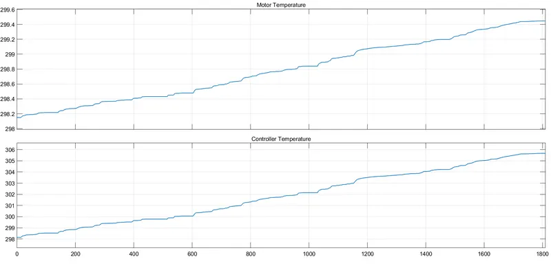
• The motor temperature rises from the initial temperature of 25°C to 26.3°C. At the same time, the temperature of the motor controller increased from 25°C to 32.5°C.

Battery Current, Battery Voltage & Battery SOC

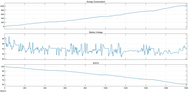
• Battery voltage fluctuates according to motor demand.
• Energy consumption is 1.01KWh, 23.26km distance covered. Battery SOC drops to 61.38%.

CONCLUSION

• Our model features a 50V, 50Ah 2.5KW battery and a 50KW PM brushed DC motor controlled by an H-bridge inverter. The body of the vehicle weighs 610 kg. Energy consumption for different drive cycles is described.
• Successfully implemented vehicle objectives and assumptions. The model was successfully simulated using 3 different drive cycles and the results were explained. The model file with the Assumptions excel file is attached.
• This is all about the basic modelling of an electric rickshaw using Simulink. We can use this simulation to see how different types of motors and controller's work. We can also add a solar panel to the Battery system. Also, we can analyse different battery performance.
• Hence, we successfully modelled an electric rickshaw (three-wheel passenger vehicle) with MATLAB and Simulink.

References

1. https://en.wikipedia.org/wiki/Electric_rickshaw

2. https://www.mordorintelligence.com/industry-reports/india-electric-rickshaw-market

3. https://www.youtube.com/watch?v=ih0UyVc6sJA