Challenge

Final Project: Design of an Electric Vehicle

AAtharva Mandale5 Jun 2021

Aim:

Create a MATLAB model of electric car which uses a battery and a DC motor. Choose suitable blocks from Powertrain block set. Prepare a report about your model including following:

Objectives:

1. System level configurations

2. Model parameters

3. Results

4. Conclusion

Introduction:

An electric vehicle (EV) is one that operates on an electric motor instead of an internal combustion engine. Therefore such a vehicle is seen as an replacement of current generation of IC engine automobiles in order to address the issue of rising pollution, global warming, depletion on natural resources, etc. Though the concept of electric vehicles has been around for a long time, it has drawn a considerable amount of interest in the past decade

Basic Block Diagram of an EV

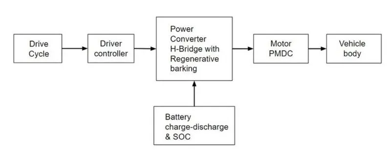
Drive cycle - This is the input given to the vehicle. This are different types of drive cycle based on the application we choose. In this vehicle is simulated for acceleration and decceleration for a particular type with the varying speed range.

Drriver Controller - To drive the drive cycle as per the given condition, a driver controller is present to run the vehicle taking the input and feedback to move from one place to another.

Power Converter - They are used to process and control the flow electric energy by supplying required voltage and current in a form that is optimally suited for the user load.

Battery - This is the power supply that provides energy required to drive the vehicle.

Vehicle Body - This is where the output is achieved via the motor power is transferred to the wheel considering the different forces and resistance and compare with input drive cycle.

Powertrain Blockset :

Powertrain Blockset provides fully assembled reference application models of automotive powertrains, including gasoline, diesel, hybrid, and electric systems. It includes a component library for simulating engine subsystems, transmission assemblies, traction motors, battery packs, and controller models. Powertrain Blockset also includes a dynamometer model for virtual testing. MDF file support provides a standards-based interface to calibration tools for data import.

Powertrain Blockset provides a standard model architecture that can be reused throughout the development process. You can use it for design tradeoff analysis and component sizing, control parameter optimization, and hardware-in-the-loop testing. You can customize models by parameterizing components in a reference application with your own data or by replacing a subsystem with your own model.

System-Level Configuration :

A. Input Circuit :

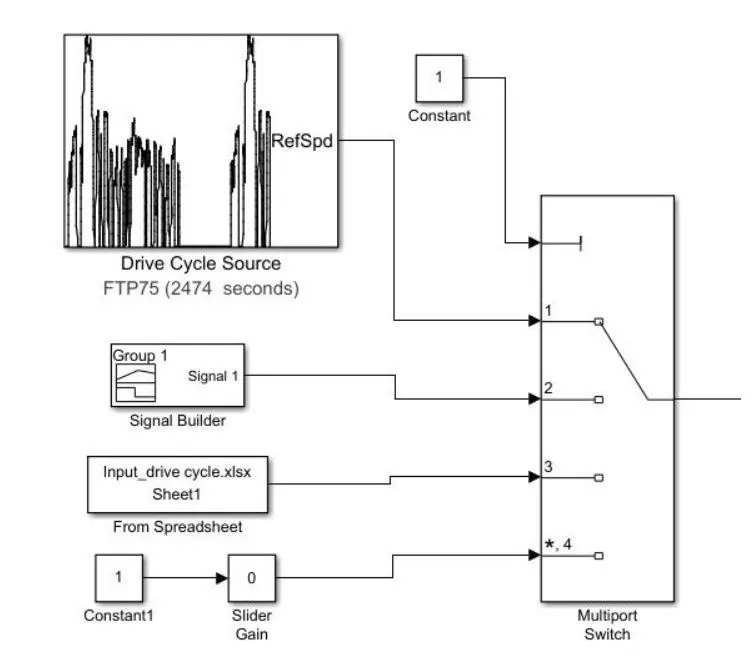
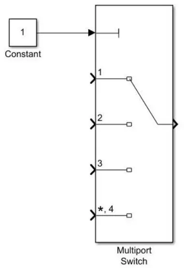
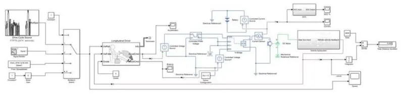
This is the input where the user defines the drive cycle and defines the behaviour of the vehicle movement for a particular time. In this, we have provided 4 different types of inputs to run the simulation of our EV model. A multiport switch is used to activate the drive cycle input has to be run for simulation by changing the value of the constant.

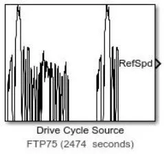
1. Drive Cycle Source :

It can generate a standard or user-specified longitudinal drive cycle. The block output is the vehicle longitudinal speed. There are different types of predefined drive cycles or can add in MATLAB workspace variables, including arrays and time series objects or spreadsheets.

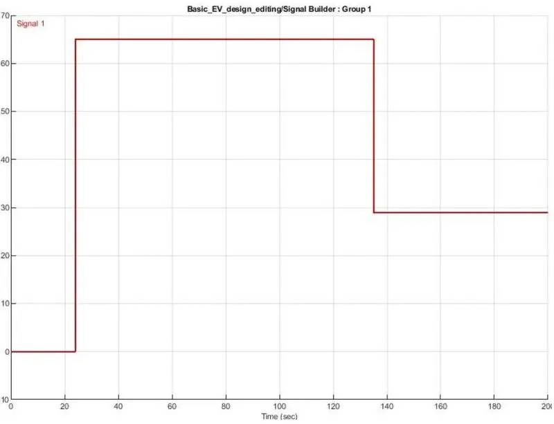
2. Signal Builder :

This block is used to create and generate interchangeable groups of signals whose waveforms are piecewise linear.

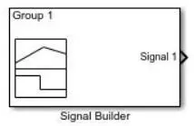
This is defined drive cycle for 200 s with acceleration at 25th sec and becoming constant after attending top speed of 65 kmph. After 135th sec the vehicle starts decceleration upto the speed of 29 kmph and becomes constant till the end of the drive cycle.

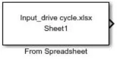
3. From Spreadsheet :

This block is called out the self-created drive cycle made in Excel sheets and use as an input.

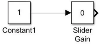
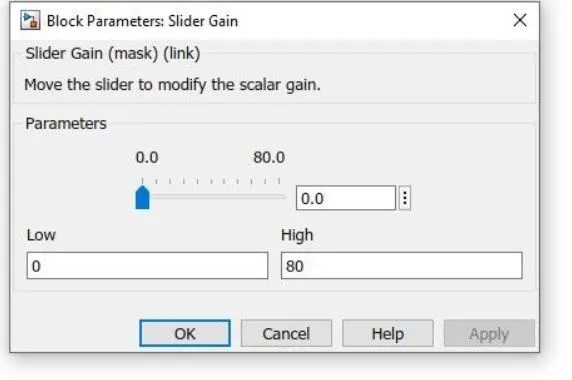
4. Slider Gain :

This block acts a slider when we can create our own drive cycle while the simulation is running by changing the position of the slider.

5. Multiport switch :

It passed through the input signals corresponding to the truncated value of the input. The inputs are numbered top to bottom, where the first input port is the control port and the other input ports are data ports.

B. Driver controller :

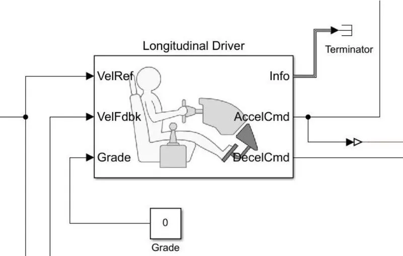
The input from the drive cycle is attached to VelRef port, the feedback is gained from the vehicle body which acts as feedback signal is connected to VelFdbk. The AccelCmd and DecelCmd are the output signal given for accelerating and braking to the vehicle. A terminator block is connected to Info port as we are not using bus signals for this model. A constant block is attached to the Grade port as road grade angle is 0 in our case, i.e. the vehicle is runnning at a straight road.

Longitudinal Drive Block :

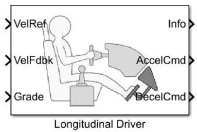
The Longitudinal Driver block implements a longitudinal speed-tracking controller. Based on reference and feedback velocities, the block generates normalized acceleration and braking commands that can vary from 0 through 1. You can use the block to model the dynamic response of a driver or to generate the commands necessary to track a longitudinal drive cycle.

Input Ports

VeRef - Reference vehicle velocity
scalar

EnblAccelOvr - Enable acceleration command override
scalar

AccelOvrCmd - Acceleration override command
scalar

AccelHld - Acceleration hold
scalar

AccelZero — Disable acceleration command
scalar

EnblDecelOvr — Enable deceleration command override
scalar

DecelOvrCmd — Deceleration override command
scalar

DecelHld — Deceleration hold
scalar

DecelZero — Disable deceleration command
scalar

ExtGear — Gear
scalar

VelFdbk — Longitudinal vehicle velocity
scalar

Grade — Road grade angle
scalar

Output

Info — Bus signal
bus

AccelCmd — Commanded vehicle acceleration
scalar

DecelCmd — Commanded vehicle deceleration
scalar

GearCmd — Commanded vehicle gear
scalar

C. Power Converters :

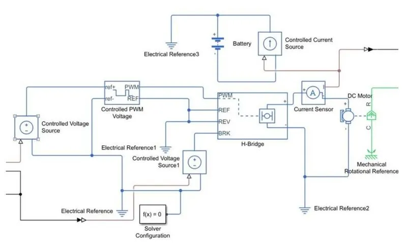
This is the min circuit where the input signals are processed and are sent at the output. The electrical power from the battery source is converted into the mechanical output of the DC motor. This block is divided into stages as follows,

1. PWM controlled voltage

The Controlled PWM Voltage block represents a pulse-width modulated (PWM) voltage source. The block has two modeling variants, accessible by right-clicking the block in your block diagram and then selecting the appropriate option from the context menu, under Simscape > Block choices:

Electrical input ports — The block calculates the duty cycle based on the reference voltage across its ref+ and ref- ports. This modeling variant is the default.
PS input — Specify the duty cycle value directly by using an input physical signal port.

For the Electrical input ports variant of the block, the demanded duty cycle is

100∗Vref−VminVmax−Vmin percent

where:

V_ref is the reference voltage across the ref+ and ref- ports.
V_min is the minimum reference voltage.
V_max is the maximum reference voltage.

The value of the Output voltage amplitude parameter determines amplitude of the output voltage.

At time zero, the pulse is initialized as high, unless the Pulse delay time parameter is greater than zero, or the demanded duty cycle is zero.

You can use parameters Pulse delay time and Pulse width offset to add a small turn-on delay and a small turn-off advance. This can be useful when fine-tuning switching times so as to minimize switching losses.

In PWM mode, the block has two options for the type of switching event when moving between output high and output low states:

Asynchronous – Best for variable-step solvers — Asynchronous events are better suited to variable step solvers, because they require fewer simulation steps for the same level of accuracy. In asynchronous mode the PWM switching events generate zero crossings, and therefore switching times are always determined accurately, regardless of the simulation maximum step size.
Discrete—time – Best for fixed-step solvers — Discrete-time events are better suited to fixed-step operation, because then the switching events are always synchronized with the simulation step. Using an asynchronous implementation with fixed-step solvers may sometimes result in events being up to one simulation step late. For more information, see Simulating with Fixed Time Step — Local and Global Fixed-Step Solvers.

If you use a fixed-step or local solver and the discrete-time switching event type, the following restrictions apply to the Sample time parameter value:

The sample time must be a multiple of the simulation step size.
The sample time must be small compared to the PWM period, to ensure sufficient resolution.

Parameters :

The PWM frequency is set to 1000 Hz and simulation mode is set to average because it also set same as in H - bridge.

The input voltage for 100 % duty cycle is kept at 5V as default value.

The output voltage amplitude is set to be at 60V for more accurate results.

2. H - Bridge

The H-Bridge block represents an H-bridge motor driver. The block has the following two Simulation mode options:

PWM — The H-Bridge block output is a controlled voltage that depends on the input signal at the PWM port. If the input signal has a value greater than the Enable threshold voltage parameter value, the H-Bridge block output is on and has a value equal to the value of the Output voltage amplitude parameter. If it has a value less than the Enable threshold voltage parameter value, the block maintains the load circuit using one of the following three Freewheeling mode options:
- Via one semiconductor switch and one freewheeling diode
- Via two freewheeling diodes
- Via two semiconductor switches and one freewheeling diode
The first and third options are sometimes referred to as synchronous operation.

The signal at the REV port determines the polarity of the output. If the value of the signal at the REV port is less than the value of the Reverse threshold voltage parameter, the output has positive polarity; otherwise, it has negative polarity.
Averaged — This mode has two Load current characteristics options:
- smoothed
- unsmoothed and discontinous
The smoothed option assumes that the current is practically continuous due to load inductance. In this case, the H-Bridge block output is:

VOVPWMAPWM−IOUTRON

where:
- V_O is the value of the Output voltage amplitude parameter.
- V_PWM is the value of the voltage at the PWM port.
- A_PWM is the value of the PWM signal amplitude parameter.
- I_OUT is the value of the output current.
- R_ON is the Bridge on resistance parameter.
The current will be smooth if the PWM frequency is large enough. Synchronous operation where freewheeling is via a bridge arm back to the supply also helps smooth the current. For cases where the current is not smooth, or possibly discontinuous (that is, it goes to zero between PWM cycles), use the unsmoothed and discontinous option. For this option, you must also provide values for the Total load series resistance, Total load series inductance, and PWM frequency. During simulation, the block uses these values to calculate a more accurate value for H-bridge output voltage that achieves the same average current as would be present if simulating in PWM mode.

Set the Simulation mode parameter to Averaged to speed up simulations when driving the H-Bridge block with a Controlled PWM Voltage block. You must also set the Simulation mode parameter of the Controlled PWM Voltage block to Averaged mode. This applies the average of the demanded PWM voltage to the motor. The accuracy of the Averaged mode simulation results relies on the validity of your assumption about the load current. If you specify that the current is Unsmoothed or discontinuous, then the accuracy also depends on the values you provide for load resistance and inductance being representative. This mode also makes some simplifying assumptions about the underlying equations for the case when current is discontinuous. For typical motor and bridge parameters, accuracy should be within a few percent. To verify Averaged mode accuracy, run the simulation using the PWM mode and compare the results to those obtained from using the Averaged mode.

Braking mode is invoked when the voltage presented at the BRK port is larger than the Braking threshold voltage. Regardless of whether in PWM or Averaged mode, when in braking mode the H-bridge is modeled by a series combination of two resistances R1 and R2 where:

R1 is the resistance of a single bridge arm, that is, half the value of the Total bridge on resistance parameter.
R2 is the resistance of a single bridge arm in parallel with a diode resistance, that is, R1 · Rd / ( R1 + Rd ), where Rd is the diode resistance.

Ports :

Port Name	Description
PWM	Input port for PWM voltage
REF	Input port for reference PWM voltage
REV	Input port for reverse signal
BRK	Input port for brake signal

Parameters :

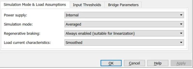
Here the power supply is keep at internal and simulation mode as average (for less run time). Regenerative braking is enabled

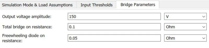
The input thresholds are kept unchanged and in the bridge parameters, the output voltage amplitude is set to 150V (but depends on the drive cycle) and rest of the parameters are unchanged

3. Controlled voltage source :

The Controlled Voltage Source block represents an ideal voltage source that is powerful enough to maintain the specified voltage at its output regardless of the current flowing through the source.

The output voltage is V = Vs, where Vs is the numerical value presented at the physical signal port.

4. DC Motor :

The DC Motor block represents the electrical and torque characteristics of a DC motor using the following equivalent circuit model:

You specify the equivalent circuit parameters for this model when you set the Model parameterization parameter to By equivalent circuit parameters. The resistor R corresponds to the resistance you specify in the Armature resistance parameter. The inductor L corresponds to the inductance you specify in the Armature inductance parameter.

You can specify how to generate the magnetic field of the DC motor by setting the Field type parameter to the desired option. The permanent magnets in the motor induce the following back emf v_b in the armature:

vb=kvω

where k_v is the Back-emf constant and ω is the angular velocity. The motor produces the following torque, which is proportional to the motor current i:

TE=kti

where k_t is the Torque constant. The DC Motor block assumes that there are no electromagnetic losses. This means that mechanical power is equal to the electrical power dissipated by the back emf in the armature. Equating these two terms gives:

TEω=vbiktiω=kvωikv=kt

As a result, you specify either k_v or k_t in the block parameters.

If the magnetic field is generated from the current flowing through the windings, the Back-emf constant depends on the field current I_f:

kv=LafIf

where L_af is the Field-armature mutual inductance.

The torque-speed characteristic for the DC Motor block is related to the parameters in the preceding figure. When you set the Model parameterization parameter to By stall torque & no-load speed or By rated power, rated speed & no-load speed, the block solves for the equivalent circuit parameters as follows:

For the steady-state torque-speed relationship, L has no effect.
Sum the voltages around the loop and rearrange for i:

i=V−vbR=V−kvωR
Substitute this value of i into the equation for torque:

TE=ktR(V−kvω)

When you set the Model parameterization parameter to By stall torque & no-load speed, the block uses the preceding equation to determine values for R and k_t (and equivalently k_v).

When you set the Model parameterization parameter to By rated power, rated speed & no-load speed, the block uses the rated speed and power to calculate the rated torque. The block uses the rated torque and no-load speed values in the preceding equation to determine values for R and k_t.

The block models motor inertia J and damping λ for all values of the Model parameterization parameter. The resulting torque across the block is:

T=ktR(V−kvω)−J˙ω−λω

It is not always possible to measure rotor damping, and rotor damping is not always provided on a manufacturer datasheet. An alternative is to use the no-load current to infer a value for rotor damping.

For no-load, the electrically-generated mechanical torque must equal the rotor damping torque:

ktinoload=λωnoload

where i_noload is the no-load current. If you select by no load current for the Rotor damping parameterization parameter, then this equation is used in addition to the torque-speed equation to determine values for λ and the other equation coefficients.

The value for rotor damping, whether specified directly or in terms of no-load current, is taken into account when determining equivalent circuit parameters for Model parameterization options By stall torque and no-load speed and By rated power, rated speed and no-load speed.

When a positive current flows from the electrical + to - ports, a positive torque acts from the mechanical C to R ports

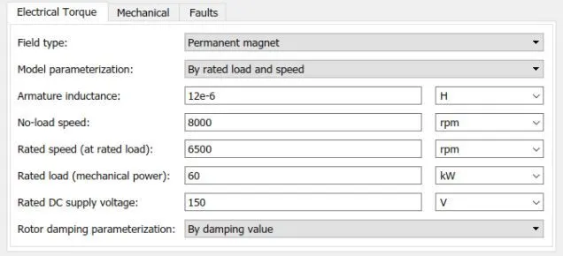
Parameters :

The model parameterization is set as by rated speed and load. The rated DC supply voltage is keep as 150 Vwhich is same as H - bridge output amplitude voltage. The speed values of the motor at no - load and rated speed is 8000 rpm and 6500 rpm simultenously. And the rated load is at 60 kW (changes as per drive cycle). The mechanical and faults parameters are kept default.

5. Battery :

The Battery block represents a simple battery model. The block has four modeling variants, accessible by right-clicking the block in your block diagram and then selecting the appropriate option from the context menu, under Simscape > Block choices:

Uninstrumented | No thermal port — Basic model that does not output battery charge level or simulate thermal effects. This modeling variant is the default.
Uninstrumented | Show thermal port — Model with exposed thermal port. This model does not measure internal charge level of the battery.
Instrumented | No thermal port — Model with exposed charge output port. This model does not simulate thermal effects.
Instrumented | Show thermal port — Model that lets you measure internal charge level of the battery and simulate thermal effects. Both the thermal port and the charge output port are exposed.

The instrumented variants have an extra physical signal port that outputs the internal state of charge. Use this functionality to change load behavior as a function of state of charge, without the complexity of building a charge state estimator.

The thermal port variants expose a thermal port, which represents the battery thermal mass. When you select this option, provide additional parameters to define battery behavior at a second temperature. For more information, see Modeling Thermal Effects.

The battery equivalent circuit is made up of the fundamental battery model, the self-discharge resistance R_SD, the charge dynamics model, and the series resistance R₀.

If you select infinity for the Battery charge capacity parameter, the block models the battery as a series resistor and a constant voltage source. If you select Finite for the Battery charge capacity parameter, the block models the battery as a series resistor and a charge-dependent voltage source. In the finite case, the voltage is a function of charge and has the following relationship:

V=V0(SOC/(1−β(1−SOC)))

where:

SOC (state-of-charge) is the ratio of current charge to rated battery capacity.
V₀ is the voltage when the battery is fully charged at no load, as defined by the Nominal voltage, Vnom parameter.
β is a constant that is calculated so that the battery voltage is V1 when the charge is AH1. Specify the voltage V1 and ampere-hour rating AH1 using block parameters. AH1 is the charge when the no-load (open-circuit) voltage is V1, and V1 is less than the nominal voltage.

The equation defines an approximate relationship between voltage and remaining charge. This approximation replicates the increasing rate of voltage drop at low charge values, and ensures that the battery voltage becomes zero when the charge level is zero. The advantage of this model is that it requires few parameters, which are readily available on most datasheets.

Parameters :

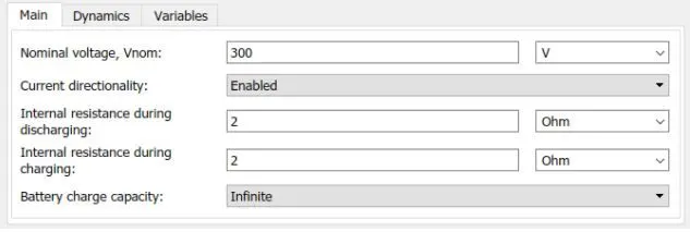
The nominal voltage is set above the DC motors rated suppy voltage and battery charge capacity is kept infinite as there will charging will regenerative braking, Rest of the parameters are default.

6. Current sensor :

The Current Sensor block represents an ideal current sensor, that is, a device that converts current measured in any electrical branch into a physical signal proportional to the current.

Connections + and – are electrical conserving ports through which the sensor is inserted into the circuit. Connection I is a physical signal port that outputs the measurement result.

7. Mechanical rotational reference :

The Mechanical Rotational Reference block represents a reference point, or frame, for all mechanical rotational ports. All rotational ports that are rigidly clamped to the frame (ground) must be connected to a Mechanical Rotational Reference block.

8. Electrical Reference :

The Electrical Reference block represents an electrical ground. Electrical conserving ports of all the blocks that are directly connected to ground must be connected to an Electrical Reference block. A model with electrical elements must contain at least one Electrical Reference block.

9. Solver configuration :

Each physical network represented by a connected Simscape™ block diagram requires solver settings information for simulation. The Solver Configuration block specifies the solver parameters that your model needs before you can begin simulation.

Each topologically distinct Simscape block diagram requires exactly one Solver Configuration block to be connected to it.

D. Vehicle body :

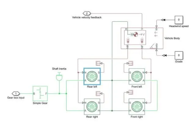
Following is the complete vehicle model using vehicle body block with 4 tire models and simple gear drive.

1. Vehicle body :

The Vehicle Body block represents a two-axle vehicle body in longitudinal motion. The vehicle can have the same or a different number of wheels on each axle. For example, two wheels on the front axle and one wheel on the rear axle. The vehicle wheels are assumed identical in size. The vehicle can also have a center of gravity (CG) that is at or below the plane of travel.

The block accounts for body mass, aerodynamic drag, road incline, and weight distribution between axles due to acceleration and road profile. Optionally include pitch and suspension dynamics. The vehicle does not move vertically relative to the ground.

The block has an option to include an externally-defined mass and an externally-defined inertia. The mass, inertia, and center of gravity of the vehicle body can vary over the course of simulation in response to system changes.

Model

The vehicle axles are parallel and form a plane. The longitudinal, x, direction lies in this plane and perpendicular to the axles. If the vehicle is traveling on an incline slope, β, the normal, z, direction is not parallel to gravity but is always perpendicular to the axle-longitudinal plane.

This figure and table define the vehicle motion model variables.

Vehicle Dynamics and Motion

Vehicle Model Variables

Symbol	Description
g	Gravitational acceleration
β	Incline angle
m	Mass of the vehicle
h	Height of vehicle center of gravity (CG) above the ground
a, b	Distance of front and rear axles, respectively, from the normal projection point of vehicle CG onto the common axle plane
V_x	Velocity of the vehicle. When V_x > 0, the vehicle moves forward. When V_x < 0, the vehicle moves backward.
V_w	Wind speed. When V_w > 0, the wind is headwind. When V_w < 0, the wind is tailwind.
n	Number of wheels on each axle
F_xf, F_xr	Longitudinal forces on each wheel at the front and rear ground contact points, respectively
F_zf, F_zr	Normal load forces on each wheel at the front and rear ground contact points, respectively
A	Effective frontal vehicle cross-sectional area
C_d	Aerodynamic drag coefficient
ρ	Mass density of air
F_d	Aerodynamic drag force

Equations

Vehicle Dynamics

The vehicle motion is a result of the net effect of all the forces and torques acting on it. The longitudinal tire forces push the vehicle forward or backward. The weight mg of the vehicle acts through its center of gravity (CG). Depending on the incline angle, the weight pulls the vehicle to the ground and pulls it either backward or forward. Whether the vehicle travels forward or backward, aerodynamic drag slows it down. For simplicity, the drag is assumed to act through the CG.

m˙Vx=Fx− Fd−mg⋅sinβ

Fx=n(Fxf+Fxr)

Fd=12CdρA(Vx+Vw)2⋅sgn(Vx+Vw)

Zero normal acceleration and zero pitch torque determine the normal force on each front and rear wheel.

Fzf=−h(Fd+mgsinβ+m˙Vx)+b⋅mgcosβn(a+b)

Fzr=+h(Fd+mgsinβ+m˙Vx)+a⋅mgcosβn(a+b)

The wheel normal forces satisfy Fzf+Fzr=mgcosβn.

If you include an externally-defined mass or inertia, the equations are shifted by the weighted value of the input.

Pitch dynamics

Pitch acceleration depends on three torque components and the inertia of the vehicle:

α=(f⋅h)+(Fzfa)−(Fzrb)J

Where:

ɑ is the pitch acceleration.
f is the longitudinal force.
h is the height of the center of gravity when measured parallel to the z-axis.
J is the inertia.

If you choose a linear model for suspension stiffness and damping, the block uses small angle approximation for pitch calculations. If you choose a table lookup model, the block uses the vectors that you specify calculate pitch dynamics. For hard stop equations, see Translational Hard Stop.

Variables

Use the Variables tab to set the priority and initial target values for the block variables before simulating. For more information, see Set Priority and Initial Target for Block Variables.

Unlike block parameters, variables do not have conditional visibility. The Variables tab lists all the existing block variables. If a variable is not used in the set of equations corresponding to the selected block configuration, the values specified for this variable are ignored.

Limitations and Assumptions

The Vehicle Body block lets you model only longitudinal dynamics, parallel to the ground and oriented along the direction of motion. The vehicle is assumed to be in pitch and normal equilibrium. The block does not model pitch or vertical movement. As such, the equations assume that the wheels never lose contact. This constraint can result in negative normal forces.

Parameters :

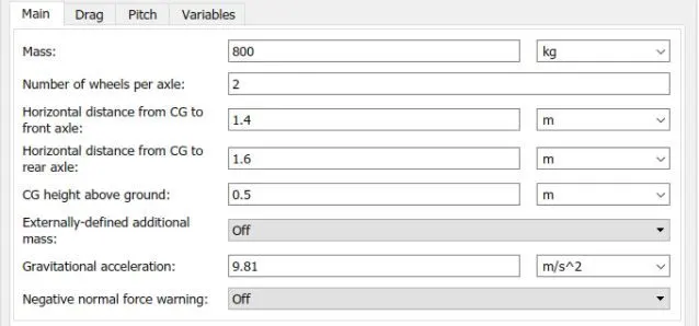
The weight of the vehicle is considered as 800 kg and rest of the parameters are same as default.

Ports :

Port Name	Description
H	It is mechanical translation converting port associated with the horizontal motion of vehicle body
NR	Signal output port for rear normal wheel force
NF	Signal output port for front normal wheel force
V	Signal output port for vehicle velocity
Beta	Signal output port for road inclination angle
W	Signal output port for headwind speed

2. Tire (Magic Formula) :

The Tire (Magic Formula) block models a tire with longitudinal behavior given by the Magic Formula [1], an empirical equation based on four fitting coefficients. The block can model tire dynamics under constant or variable pavement conditions.

The longitudinal direction of the tire is the same as its direction of motion as it rolls on pavement. This block is a structural component based on the Tire-Road Interaction (Magic Formula) block.

To increase the fidelity of the tire model, you can specify properties such as tire compliance, inertia, and rolling resistance. However, these properties increase the complexity of the tire model and can slow down simulation. Consider ignoring tire compliance and inertia if simulating the model in real time or if preparing the model for hardware-in-the-loop (HIL) simulation.

Parameters :

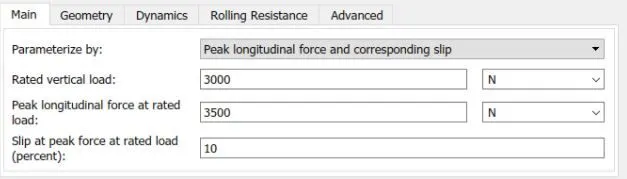
The tire is parameterized by peak longitudinal force and corresponding slip and rest pf the parameters are kept default.

Ports :

Port Name	Description
N	Signal input port that applies the normal force acting on the tire
A	It is the mechanical rotational conserving port for the wheel axle
S	Signal output port that reports the tire slip
H	It is the mechanical translational conserving port for the wheel hub

3. Simple Gear :

The Simple Gear block represents a gearbox that constrains the connected driveline axes of the base gear, B, and the follower gear, F, to corotate with a fixed ratio that you specify. You choose whether the follower axis rotates in the same or opposite direction as the base axis. If they rotate in the same direction, the angular velocity of the follower, ω_F, and the angular velocity of the base, ω_B, have the same sign. If they rotate in opposite directions, ω_F and ω_B have opposite signs.

Parameters :

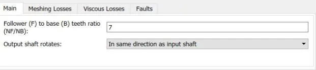
Here we have set gear ratio as 7. As torque is directly proportional to the speed. The gear ratio is high at the start of the vehicle as it requires more torque and as the speed increases, torque reduces and so does the gear ratio.

Port :

Port Name	Description
B	Input signal for mechanical rotational conserving port from DC motor
F	Output signal for mechanical rotational conserving port after gear reduction

4. Shaft Inertia :

The Inertia block represents an ideal mechanical translational inertia that is described with the following equation:

T=Jdω/dt

where:

T is inertia torque.
J is inertia.
ω is angular velocity.
t is time.

By default, the block has one mechanical translational conserving port. The block positive direction is from its port to the reference point. This means that the inertia torque is positive if inertia is accelerated in the positive direction.

In some applications, it is customary to display inertia in series with other elements in the block diagram layout. To support this use case, the Number of graphical ports parameter lets you display a second port on the opposite side of the block icon. The two-port variant is purely graphical: the two ports have the same angular velocity, so the block functions exactly the same whether it has one or two ports.

E. State of charge (SOC) :

This will determine the voltage level in the battery at eacch point of simulation. The output from the current block is received at the input signal of the block and display the characteristic of the battery voltage consumed for the particular drive cycle.

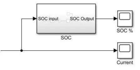
The sub-block of the SOC contains the Rate transition block, gain block and the discrete time ingegrator. The decrease and increase of the battery voltage have multiple data point which is handled by the rate transistors. Then this converts these data points calculate the SOC at each point of the drive cycle. The gain block will calulate the values and display on the scope.

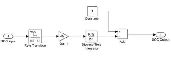
Equation -

K = 1 / V_rated x Time

where, time is 3600 sec and multiplication is element-wise

1. Rate Transition :

It handles data transfer between different rates and task

2. Gain :

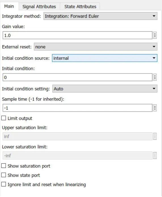
3. Discrete-time Integration :

Parameter :

F. Output Circuit :

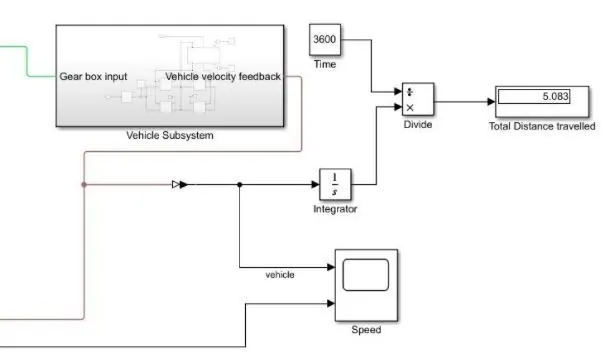
The output of the vehicle body is velocity which is sent as feedback to the longitudinal drive block and is seperately used to calculate the distance travelled by the vehicle through another subsystem - distance calculator.

The velocity signal is first integrated to calculate the distance and then divide by 3600 to convert distance to km.

Complete EV Model :

RESULTS :

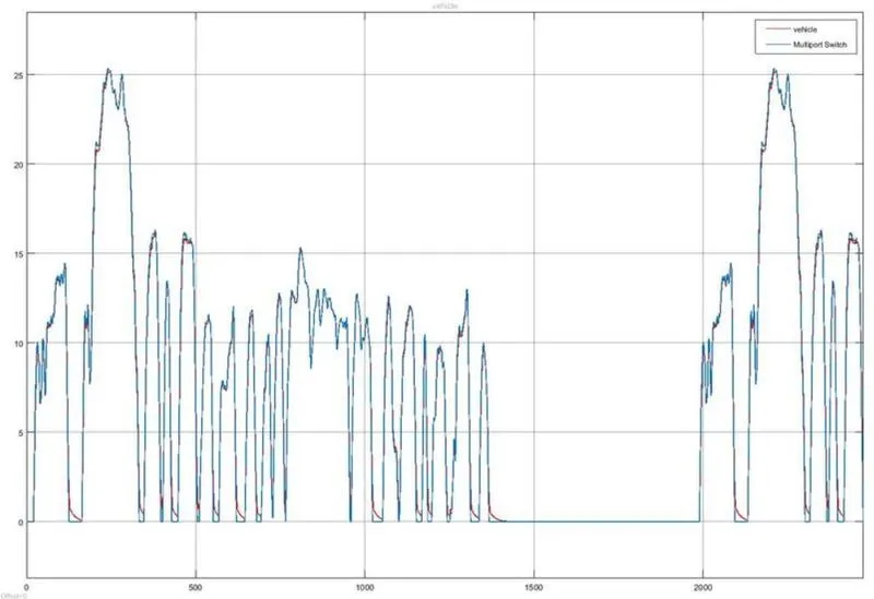
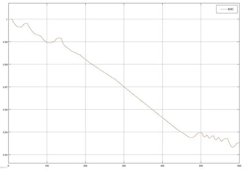
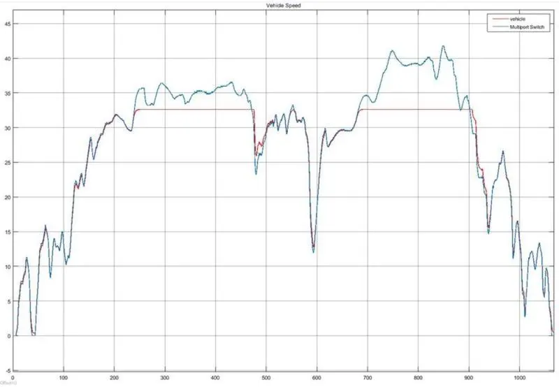
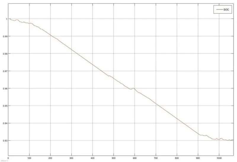
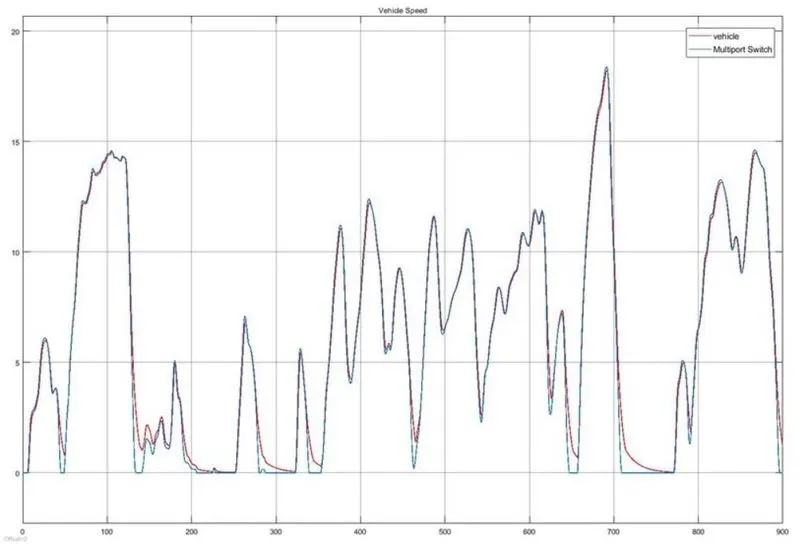
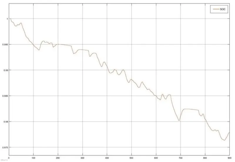
The simulations are run for various drive cycles and the results are in the following table

	Case 1	Case 2	Case 3	Case 4
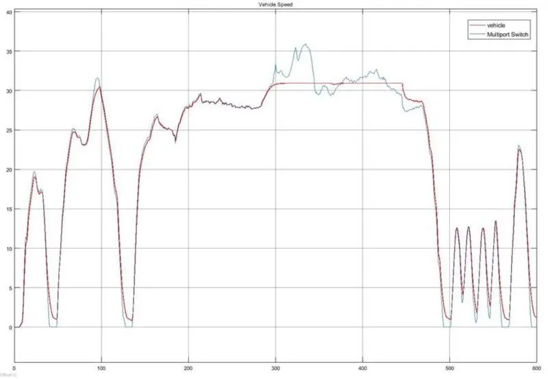
Drive cycle simulation time (s)	FTP75, 2474	US06,600	Artemis motorway 150kmph,1068	World Harmonized vehicle cycle(WHVC),900
Vehicle body wt. (kg), frontal area (m^2), Drag Coefficient, Rolling resistance	800,3,0.4,0.015	800,3,0.4,0.015	800,3,0.4,0.015	800,3,0.4,0.015
Battery Nominal Voltage (V)	300	300	400	200
DC Motor Rated load (kW), Rated Voltage (V)	60,300	75,200	85,350	60,150
H-Bridge Output voltage amplitude	300	200	350	150
Distance (km),Top speed (kmph)	4.97,25.2	3.54,30.8	7.77,32.6	1.52,18.2
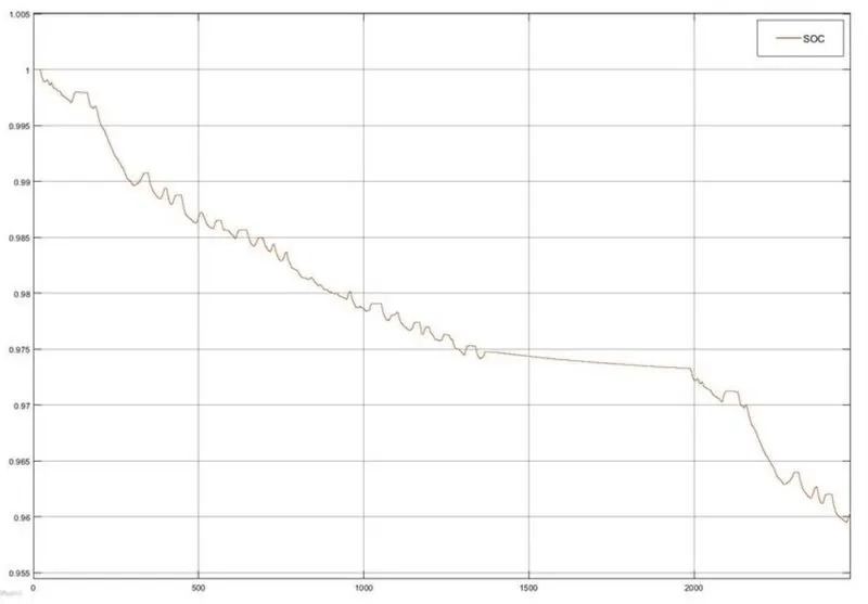
SoC at the end of drive cycle (ini. SoC = 100%)	96	94	93	97
Top speed reached? kWh per km	Yes	No	No	Yes

Output Graphs :

A. Case - 1

1. Speed Characteristics :

2. SOC (%) :

B. Case - 2

1. Speed Characteristics :

2. SOC (%)

C. Case - 3

1. Speed Characteristics :

2. SOC (%)

D. Case - 4

1. Speed Characteristics :

2. SOC (%)

Conclusion :

In the speed trace plot for all the drive cycles which are observed in this study, the feedback speed plot and the reference speed plot overlap each other almost completely but there are regions where both the speeds are different. It is when the vehicle is deceleration.
The reference speed plot falls sharply but the feedback speed does not. This is due to the inertia of the vehicle body. As the inertia of the vehicle body is higher, it takes a longer duration for it to decelerate. That is why the overlapping is not 100%.
The battery's state of charge for each drive cycle can be visualized from the SOC plot. As long as the vehicle is accelerating the SOC is decreasing but as soon as the deceleration starts, the SOC plot goes slightly up. This is because the battery is being charged, due to regenerative braking during deceleration.

Link - https://drive.google.com/file/d/1YngDdpUkWn2HXdgi28ova6EvxltqxS9s/view?usp=sharing