Final Project: Design of an Electric Vehicle

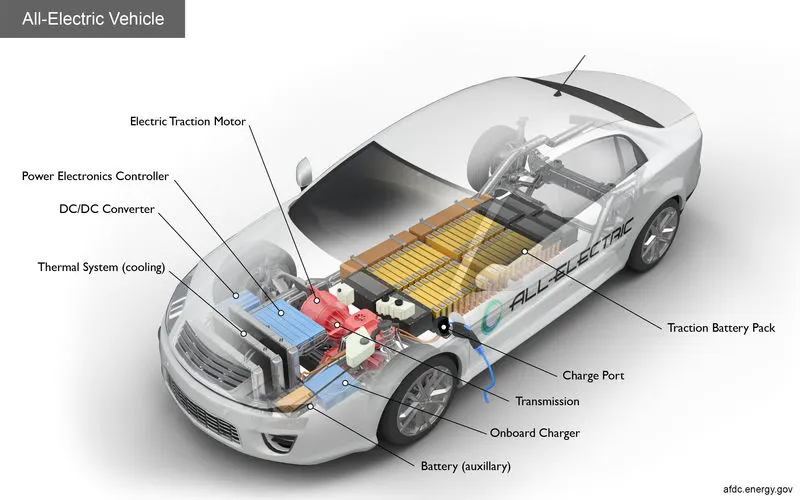
• Battery (all-electric auxiliary): In an electric drive vehicle, the auxiliary battery provides electricity to power vehicle accessories.
• Charge port: The charge port allows the vehicle to connect to an external power supply to charge the traction battery pack.
• DC/DC converter: This device converts higher-voltage DC power from the traction battery pack to the lower-voltage DC power needed to run vehicle accessories and recharge the auxiliary battery.
• Electric traction motor: Using power from the traction battery pack, this motor drives the vehicle's wheels. Some vehicles use motor generators that perform both the drive and regeneration functions.
• Onboard charger: Takes the incoming AC electricity supplied via the charge port and converts it to DC power for charging the traction battery. It also communicates with the charging equipment and monitors battery characteristics such as voltage, current, temperature, and state of charge while charging the pack.
• Power electronics controller: This unit manages the flow of electrical energy delivered by the traction battery, controlling the speed of the electric traction motor and the torque it produces.
• Thermal system (cooling): This system maintains a proper operating temperature range of the engine, electric motor, power electronics, and other components.
• Traction battery pack: Stores electricity for use by the electric traction motor.
• Transmission (electric): The transmission transfers mechanical power from the electric traction motor to drive the wheels.

Block diagram of the model:

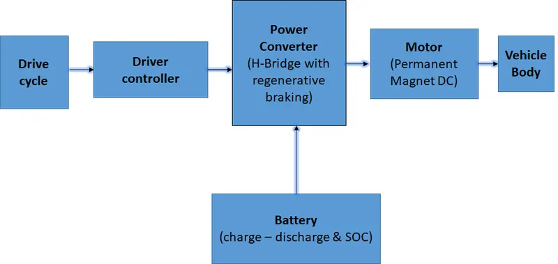
Block diagram of Powertrain of EV

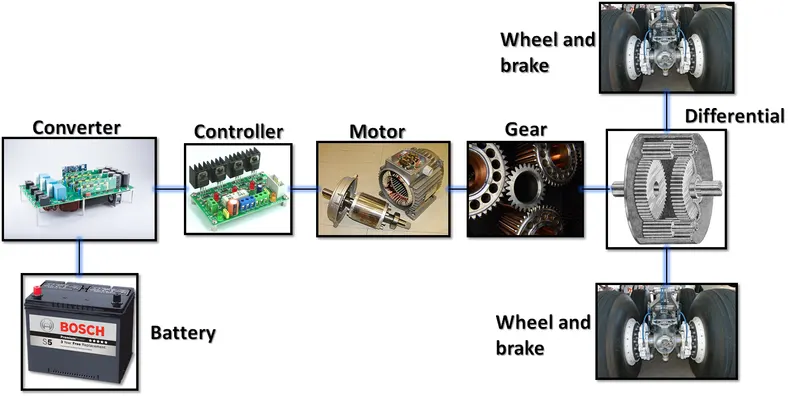
the Model is as shown:

CLICK HERE TO GET THE BELOW MATLAB MODEL

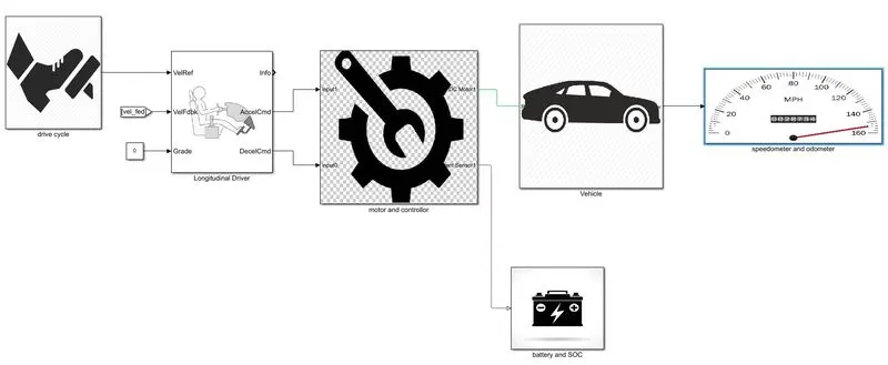
Drive cycle :

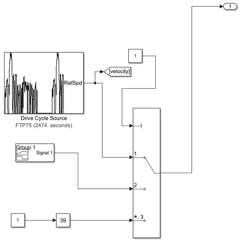
The Drive Cycle Source block generates a standard or user-specified longitudinal drive cycle. The block output is the specified vehicle longitudinal speed.

1. drive cycle source(FTP75): this is the Matlab built-in drive cycle that gives desired output speed to the driver which compares this with the current speed and produces an error.
2. signal builder: this drive cycle is made by the user by choosing the appropriate speed he wants at the instant.
3. slider gain: using this block you can control the speed of the vehicle by adjusting the slider.

here, The Multiport Switch block determines which of several inputs to the block passes to the output. The block bases this decision on the value of the first input. The first input is the control input and the remaining inputs are the data inputs. The control input value determines which data input passes to the output.

Driver:

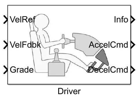
Inputs:

• VelRef: takes the input from the drive cycle.
• VelFdbk: takes the input from the velocity of the vehicle and compares it with the reference velocity here there will be an error signal if the signal is a positive error then the driver block will give a signal to the accelCmd to increase and vice versa.
• Grade: indicates the % of the gradeability i.e the angle of slope.
• AccelCmd: this output is given to the controlled PWM voltage to process the PWM signal, which is connected to the H-bridge input PWM to control speed and torque.
• DecelCmd: this output is directly given to the BRK input of the H-bridge.

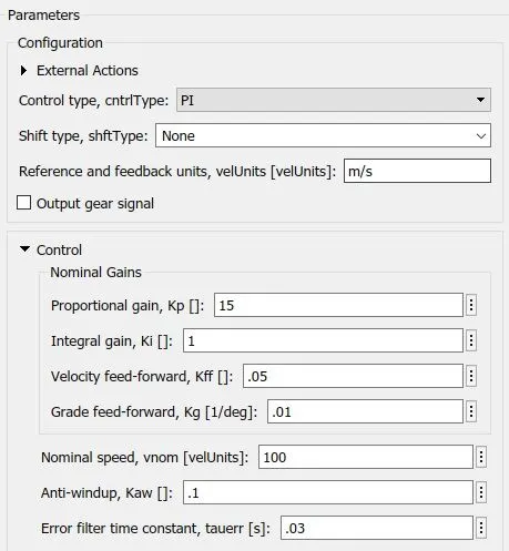
A parametric longitudinal speed tracking controller for generating normalized acceleration and braking commands based on reference and feedback velocities.

Use the external actions to input signals that can disable, hold, or override the closed-loop commands determined by the block. The block uses this priority for the input commands: disable, hold, override.

Motor and Controller Subsystem:

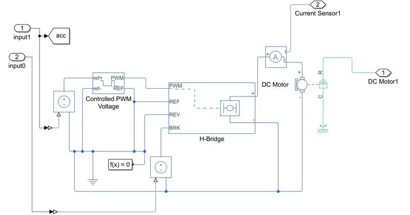
The input to this system is given by the longitudinal driver the two inputs are acceleration and deceleration command depending upon the desired speed and torque.

• acceleration command input is given to controlled PWM voltage via a controlled voltage source to process the PWM signal, which is connected to the H-bridge input PWM to control speed, and torque
• deceleration command is directly given to the BRK input of the H-bridge via controlled voltage source.
• solver configuration block specifies the solver parameters that your model needs before you can begin the simulation. Each topologically distinct Simscape block diagram requires exactly one Solver Configuration block to be connected to it.
• H-bridge is connected here this is a power converter that regulates voltage to control the speed and torque of the DC motor and hence the two terminals are connected to the motor as shown above.
• The Current Sensor block represents an ideal current sensor, that is, a device that converts current measured in any electrical branch into a physical signal proportional to the current. Connections + and – are electrical conserving ports through which the sensor is inserted into the circuit. The connection is a physical signal port that outputs the measurement result.
• the current sensor output is given to the battery subsystem.
• the DC-motor output is given to the vehicle body i.e the power is given to the transmission and gear system to perform the desired condition.

H-Bridge

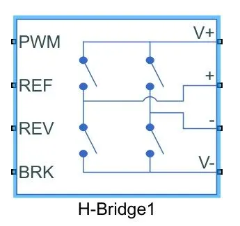
This block represents an H-bridge motor drive. The block can be driven by the Controlled PWM Voltage block in PWM or Averaged mode. In PWM mode, the motor is powered if the PWM port voltage is above the Enable threshold voltage. In Averaged mode, the PWM port voltage divided by the PWM signal amplitude parameter defines the ratio of the on-time to the PWM period. Using this ratio and assumptions about the load, the block applies an average voltage to the load that achieves the correct average load current. The Simulation mode parameter value must be the same for the Controlled PWM Voltage and H-Bridge blocks.

If the REV port voltage is greater than the Reverse threshold voltage, then the output voltage polarity is reversed. If the BRK port voltage is greater than the Braking threshold voltage, then the output terminals are short-circuited via one bridge arm in series with the parallel combination of a second bridge arm and a freewheeling diode. Voltages at ports PWM, REV, and BRK are defined relative to the REF port.

DC-motor:

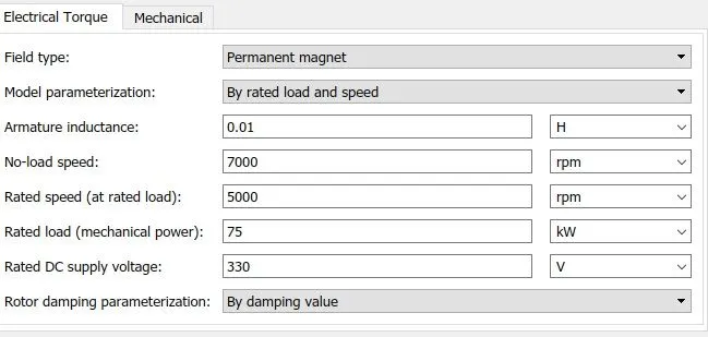
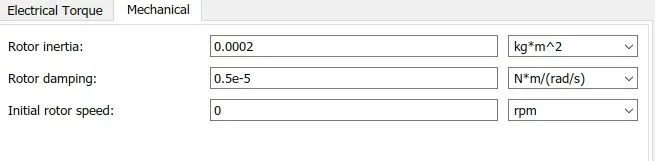
This block represents the electrical and torque characteristics of a DC motor. The block assumes that no electromagnetic energy is lost, and hence the back-emf and torque constants have the same numerical value when in SI units. Motor parameters can either be specified directly or derived from the no-load speed and stall torque. If no information is available on armature inductance, this parameter can be set to some small non-zero value. When a positive current flows from the electrical + to - ports, a positive torque acts from the mechanical C to R ports. Motor torque direction can be changed by altering the sign of the back-emf or torque constants.

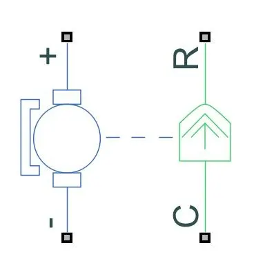
The resulting torque across the block is:

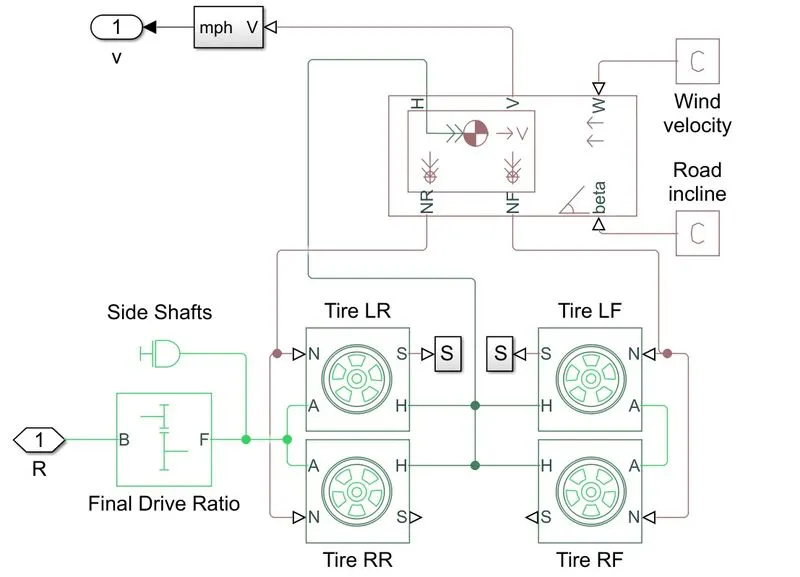
• the gears are connected to the wheels' transmission.
• the tire hubs are connected to the vehicle body.
• this vehicle is a rear-wheel drive and hence the power that is transmitted through gears is given to the real tired only.
• a moment inertia block is also given to the gear system since there will be initial inertia during the start of the vehicle.

vehicle body:

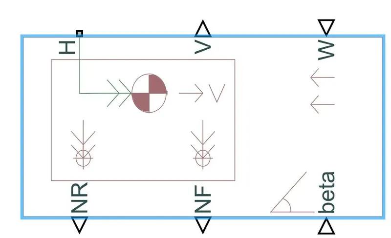
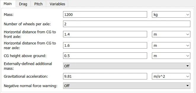
Represents a two-axle vehicle body in longitudinal motion. The block accounts for body mass, aerodynamic drag, road incline, and weight distribution between axles due to acceleration and road profile. The vehicle can have the same or different wheels on each axle. Optionally include pitch and suspension dynamics or additional variable mass and inertia. The vehicle does not move vertically relative to the ground.

Connection H is the mechanical translational conserving port associated with the horizontal motion of the vehicle body. The resulting traction motion developed by tires should be connected to this port. Connections V, NF, and NR are physical signal output ports for vehicle velocity and front and rear normal wheel forces. Wheel forces are considered positive if acting downwards. Connections W and beta are physical signal input ports corresponding to headwind speed and road inclination angle. If the variable mass is modeled, the physical signal input ports CG and M are exposed. CG accepts a two-element vector representing the x and y distance offsets from vehicle CG to additional load mass CG. M represents the additional mass. If both variable mass and pitch dynamics are included, the physical signal port J accepts the inertia of the additional mass about its own CG.

Tire:

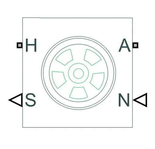
Represents the longitudinal behavior of a highway tire characterized by the tire Magic Formula. The block is built from Tire-Road Interaction (Magic Formula) and Simscape Foundation Library Wheel and Axle blocks. Optionally, the effects of tire inertia, stiffness, and damping can be included.

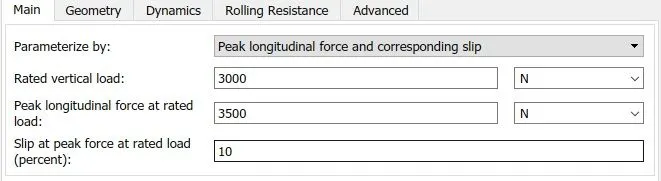
Connection A is the mechanical rotational conserving port for the wheel axle. Connection H is the mechanical translational conserving port for the wheel hub through which the thrust developed by the tire is applied to the vehicle. Connection N is a physical signal input port that applies the normal force acting on the tire. The force is considered positive if it acts downwards. Connection S is a physical signal output port that reports the tire slip. Optionally expose physical signal port M by setting Parameterize by to Physical signal Magic Formula coefficients. Physical signal port M accepts a four-element vector corresponding to the B, C, D, and E Magic Formula coefficients.

Battery and SOC Subsystem:

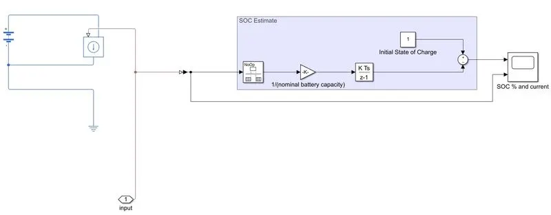
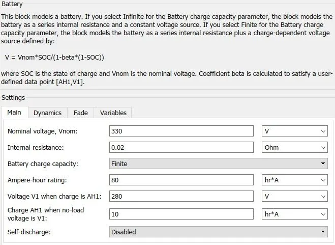
for the power source, we have used a battery source block which disconnected to a constant block. When we double click on Battery block we get the following box

SOC Estimate:

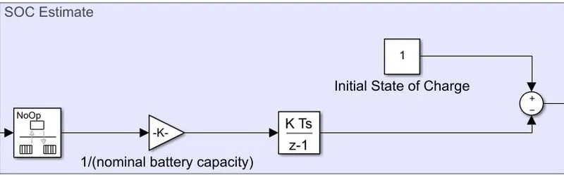
This block estimates the batter SOC% using the coulomb counting method. It takes current as the input and gives SOC% as output. The initial SOC of the battery is assumed to be 100%. And while calculating the SOC, battery capacity is assumed to be 100Ah.

Simulation and its results:

the measurement block is as follows:

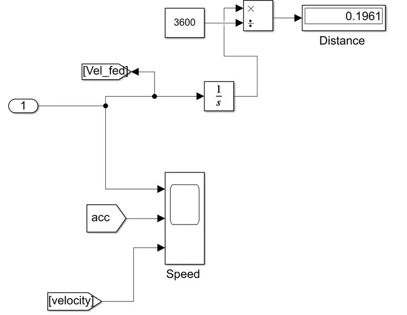
The FTP75 drive cycle is given as a speed reference to the driver. The FTP cycle (for Federal Test Procedure) has been created by US EPA (Environmental Protection Agency) to represent a commuting cycle with a part of urban driving including frequent stops and a part of highway driving. this cycle covers a distance of 17.77 Km in 2474 seconds. note it has a top speed of 90km/hr

Run time is 2472 seconds:

the below image shows the reference speed or the desired speed of the drive cycle and the vehicle actual speed with respect to time. Achieved using the model.

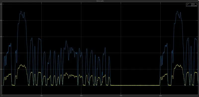
• The main reason for the plot to not follow the reference speed is due to inertia of the vehicle which is high this is the reason with heavy vehicles they wont be able to achieve the speed required in shorter amount of time
• we can observe that the top speed of 26.78km/hr.
• and also follows the reference speed but not so well during the whole cycle. Some deviations are there because of the instant change in the reference speed which would be hard braking or high acceleration.
• when we look closely the deviations are mainly due to braking that is the reason in modern cars there is a warning for the sudden brakes because the motor is getting is the strain it affected due to this.
• and also the main reason for this effect is that we are not using mechanical brakes we are only regenerative braking and this is the reason electric cars can be driven using only the single pedal
• and also the actual distance covered is also close to the drive cycle distance.

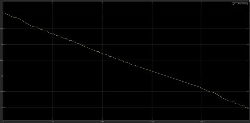
After the simulation, battery SOC is reduced to 67.18% from 100% initial SOC, As the vehicle starts moving, battery SOC also starts to reduce and when the brake is applied we cans ee the SOC slightly increases as the battery is charged due to the regenerative braking, And during the time vehicle is at rest, battery SOC is not constant because the motor is using the energy to stop the vehicle since there is huge inertia.

So, we can observe that vehicle uses about 33% of the total battery capacity to travel a distance of 5.59Km because the inertia of the vehicle is more that is the reason when you require torque you reduce the speed of the vehicle to achieve the torque in order to provide the torque required the vehicle as to increase the voltage supply and current and hence we will get shorter distance for more usage of power.