Final Project: Design of an Electric Vehicle
Aim: To create a MATLAB model of an electric car which uses a DC motor by choosing suitable blocks from the Powertrain block set.
Objectives: To prepare a report about the model which discusses the following:
1. System level configurations
2. Model parameters
3. Results
4. Conclusion
Theory:
The use of fossil fuels for energy has been a practice for centuries, leading not only to the depletion of these resources but also to the release of greenhouse gases (GHGs) as a harmful byproduct. These emissions have significantly contributed to global climate change, as seen in the rising temperatures. To address these challenges, efforts are being made to develop alternative fuels and incorporate cleaner technologies in vehicles, aiming to reduce GHG emissions while improving vehicle performance. A key strategy in this transition is the electrification of transportation through the adoption of Electric Vehicles (EVs). EVs have the potential to diversify energy sources, drive economic growth by creating advanced industries and most importantly, reduce emissions, thereby helping to protect the environment [1]. An electric vehicle (EV) is a vehicle which uses an electric motor for propulsion. It can be categorized into hybrid electric vehicles (HEVs), plug-in hybrid electric vehicles (PHEVs) and battery electric vehicles (BEVs).
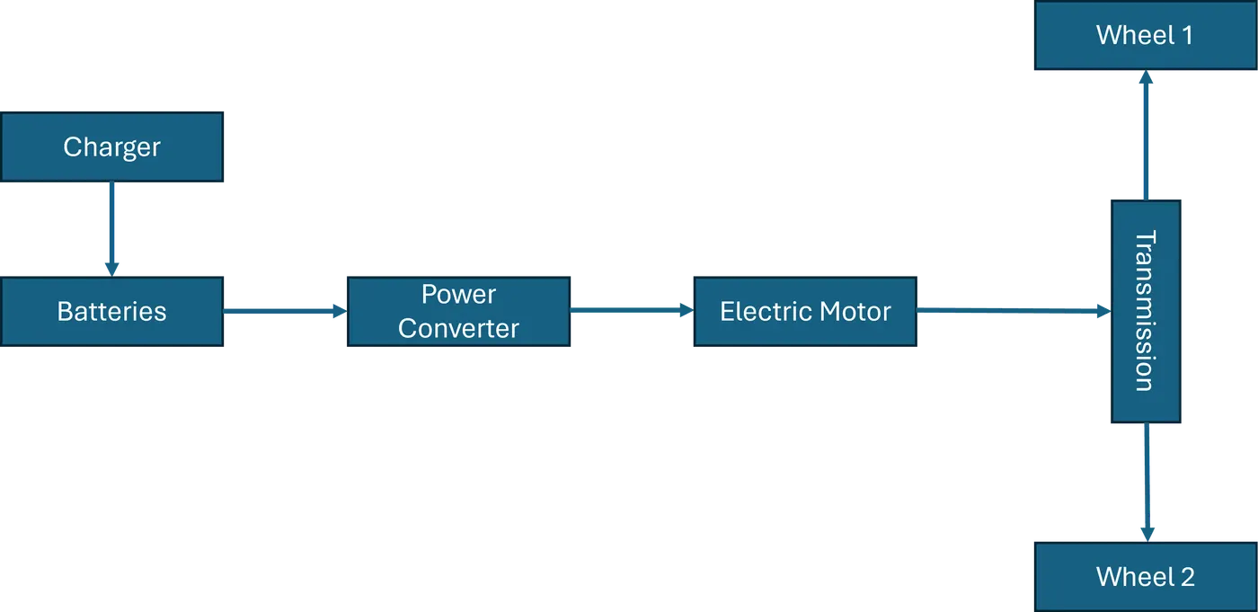
The basic components of EV consists of:
1. Battery
2. Power Converter
3. Electric motor
4. Transmission
Other components, such as the fuel tank and Internal Combustion Engine (ICE), are also included in HEVs and chargers are included in PHEVs. To further improve efficiency, the batteries are charged through ICE using a generator or through an energy recovery mechanism called regenerative braking.
A typical power train configuration of BEV is shown below [1],
Modelling Electric Vehicles (EVs) using simulation tools is crucial, as it enables the execution of various drive cycles, testing of different battery types, and analysis of key characteristics such as range and State of Charge (SOC). This approach allows for the comparison of different options, aiding in the selection of suitable motors and batteries during the early stages of the design process.
Simulink model of Electric Vehicle:
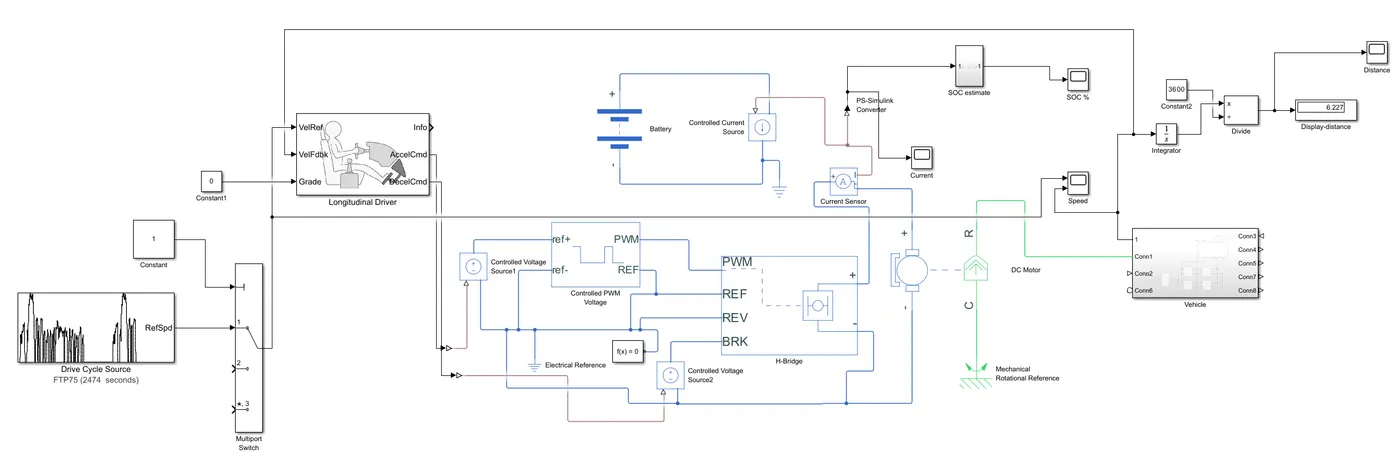
Simulink blocks used are as follows:
1. Drive Cycle Source
2. Multiport switch
3. Longitudinal Driver
4. Controlled PWM Voltage
5. H-Bridge
6. DC Motor
7. Battery
8. Controlled Voltage Source
9. Controlled Current Source
10. Current Sensor
11. Vehicle Body
12. Simple Gear
13. Tire (magic formula)
14. Constant
15. Product
16. Sum
17. Gain
18. Electrical Resistance
19. Mechanical Rotational Resistance
20. Display
21. Scope
22. PS-Simulink and Simulink-PS converters
23. Integrator
Block Parameters
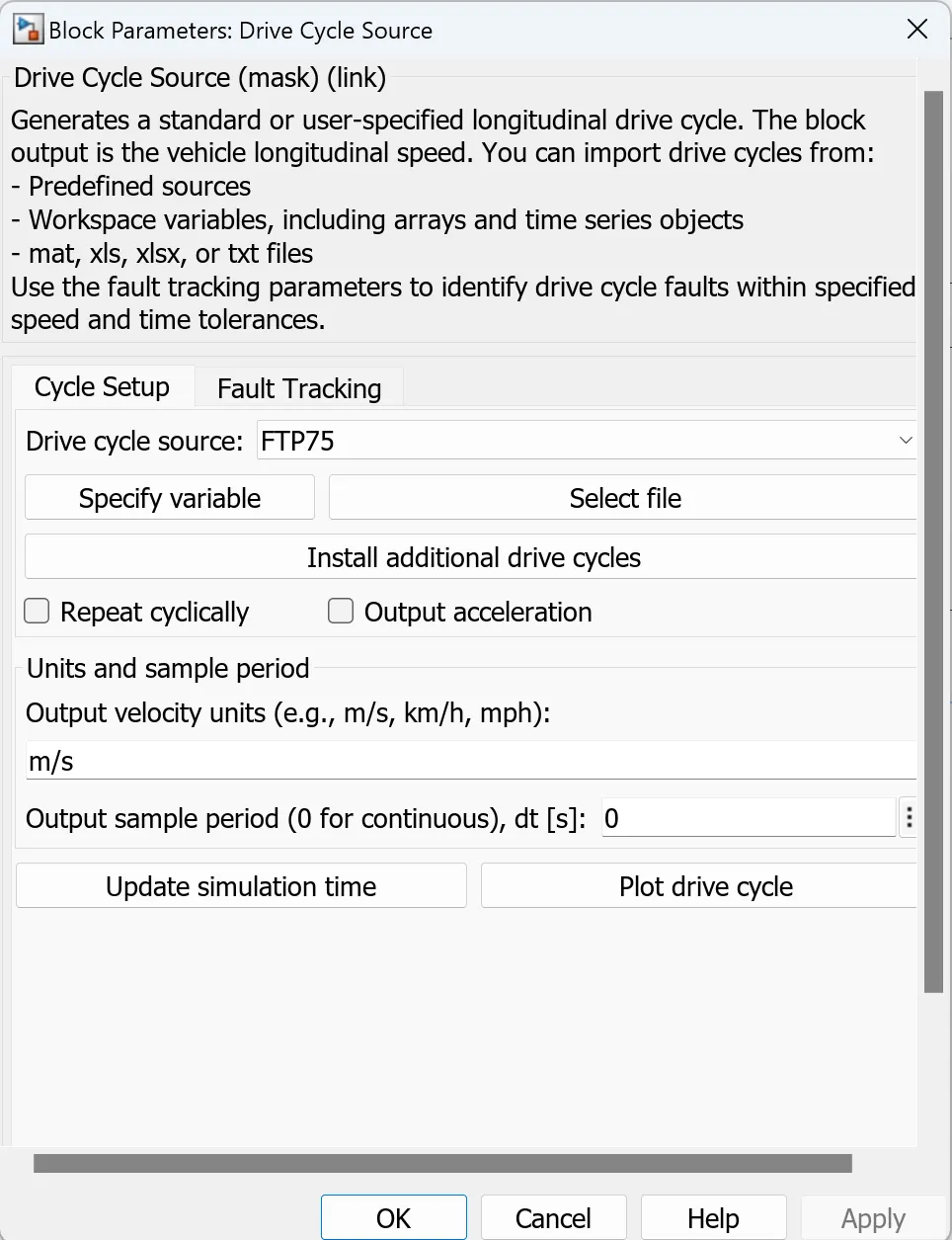
1. Drive Cycle Source
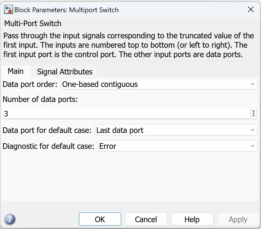
2. Multiport switch
3. Longitudinal Driver
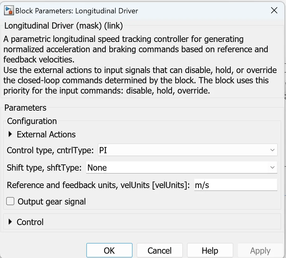
4. Controlled PWM Voltage
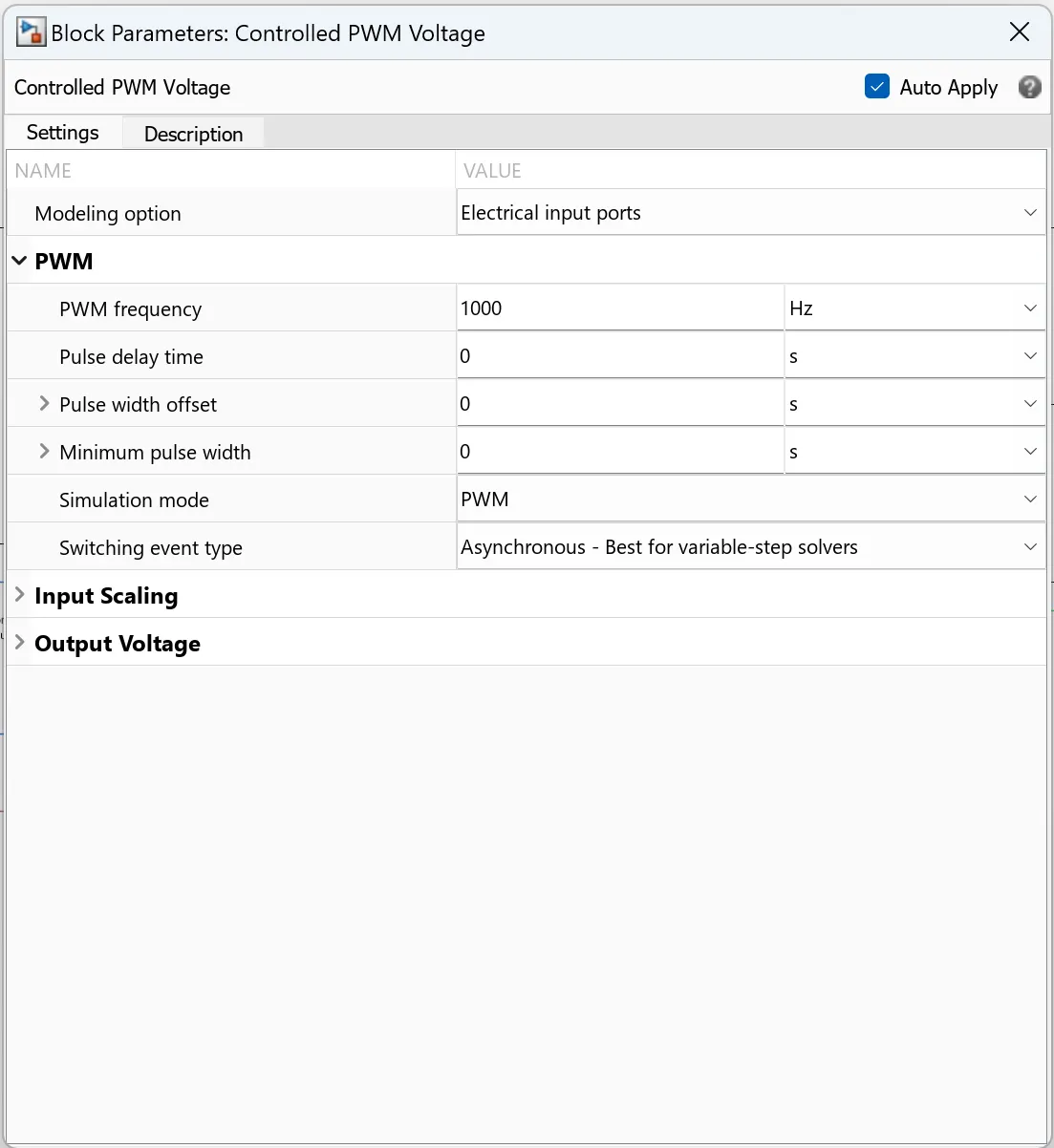
5. H-Bridge
This block represents an H-bridge motor drive, which can be controlled using the Controlled PWM Voltage block in either PWM or Averaged mode. In PWM mode, the motor is activated when the PWM port voltage exceeds the Enable threshold voltage. In Averaged mode, the ratio of the PWM port voltage to the PWM signal amplitude parameter determines the proportion of the on-time relative to the PWM period. Based on this ratio and assumptions about the load, the block applies an average voltage that ensures the correct average current through the load. The Simulation mode parameter must match between the Controlled PWM Voltage block and the H-Bridge block for proper operation.
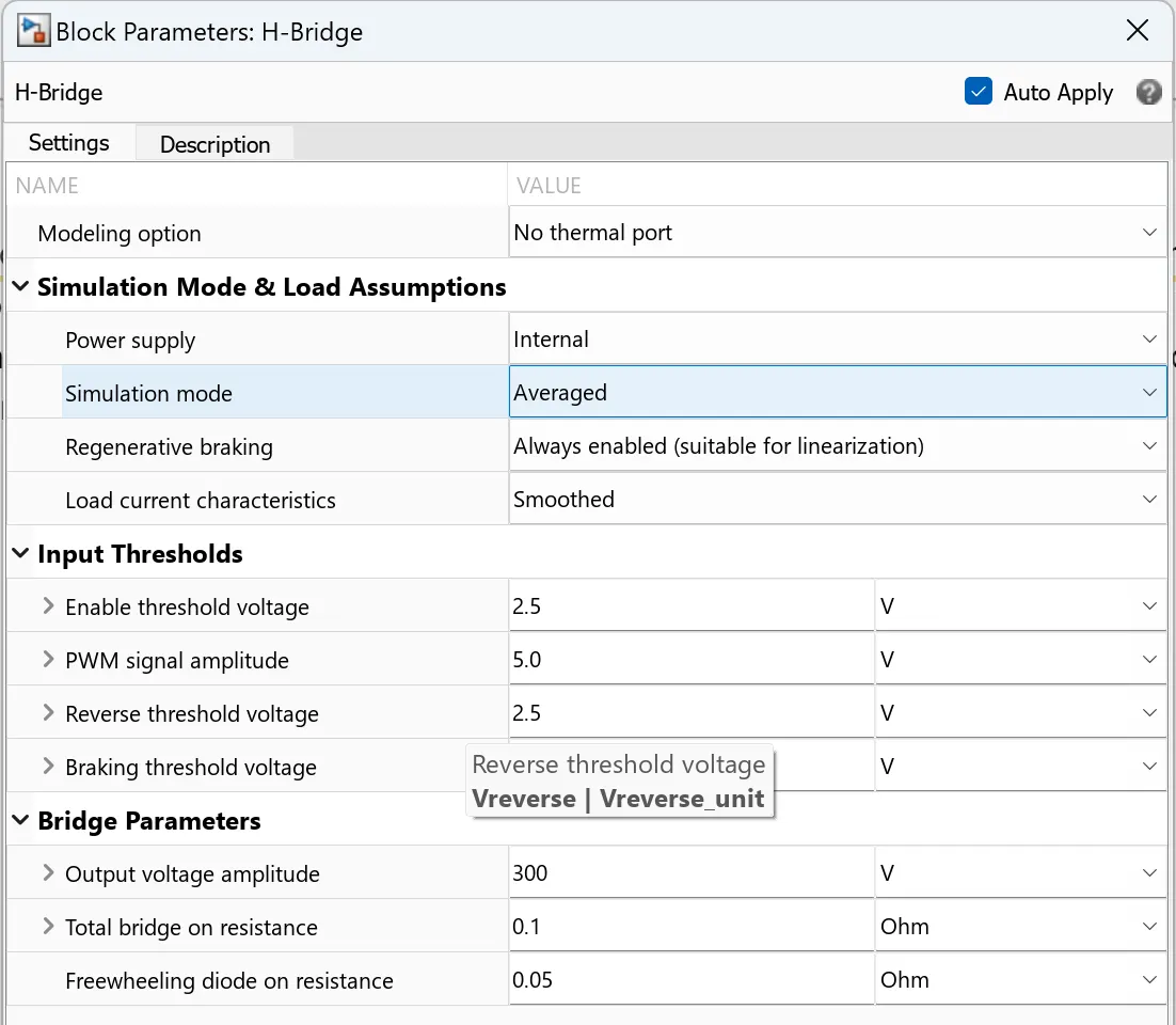
6. DC Motor
7. Battery
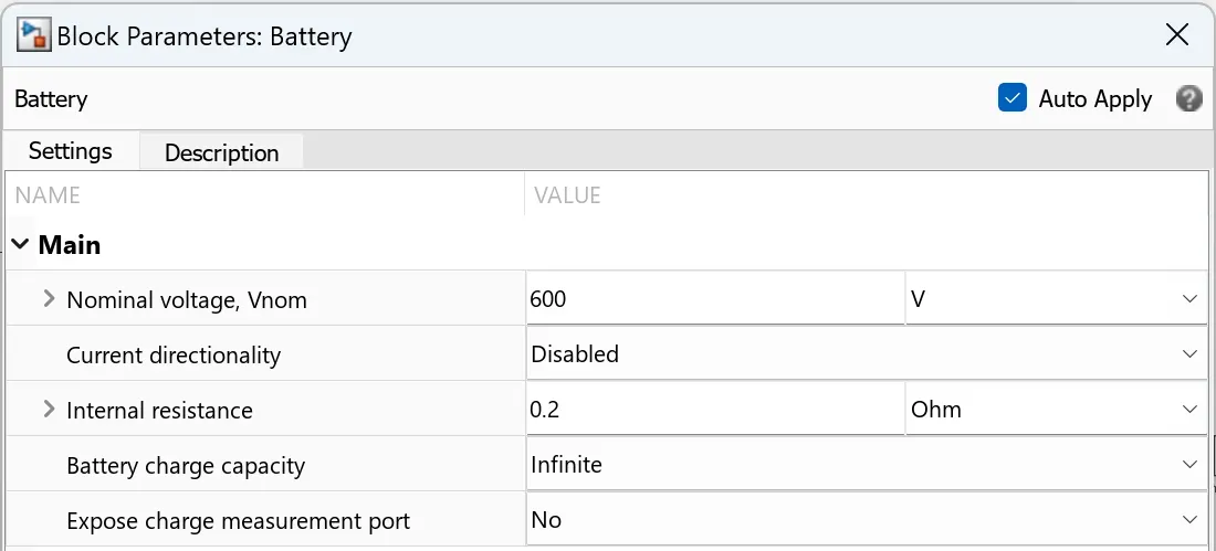
This block models a battery. If you set the Battery charge capacity parameter to Infinite, the block models the battery as a series internal resistance and a constant voltage source. If you set the Battery charge capacity parameter to Finite, the block models the battery as a series internal resistance plus a charge-dependent voltage source defined by:
V = Vnom*SOC/(1-beta*(1-SOC))
where SOC is the state of charge and Vnom is the nominal voltage. Coefficient beta is calculated to satisfy a user-defined data point [AH1,V1].
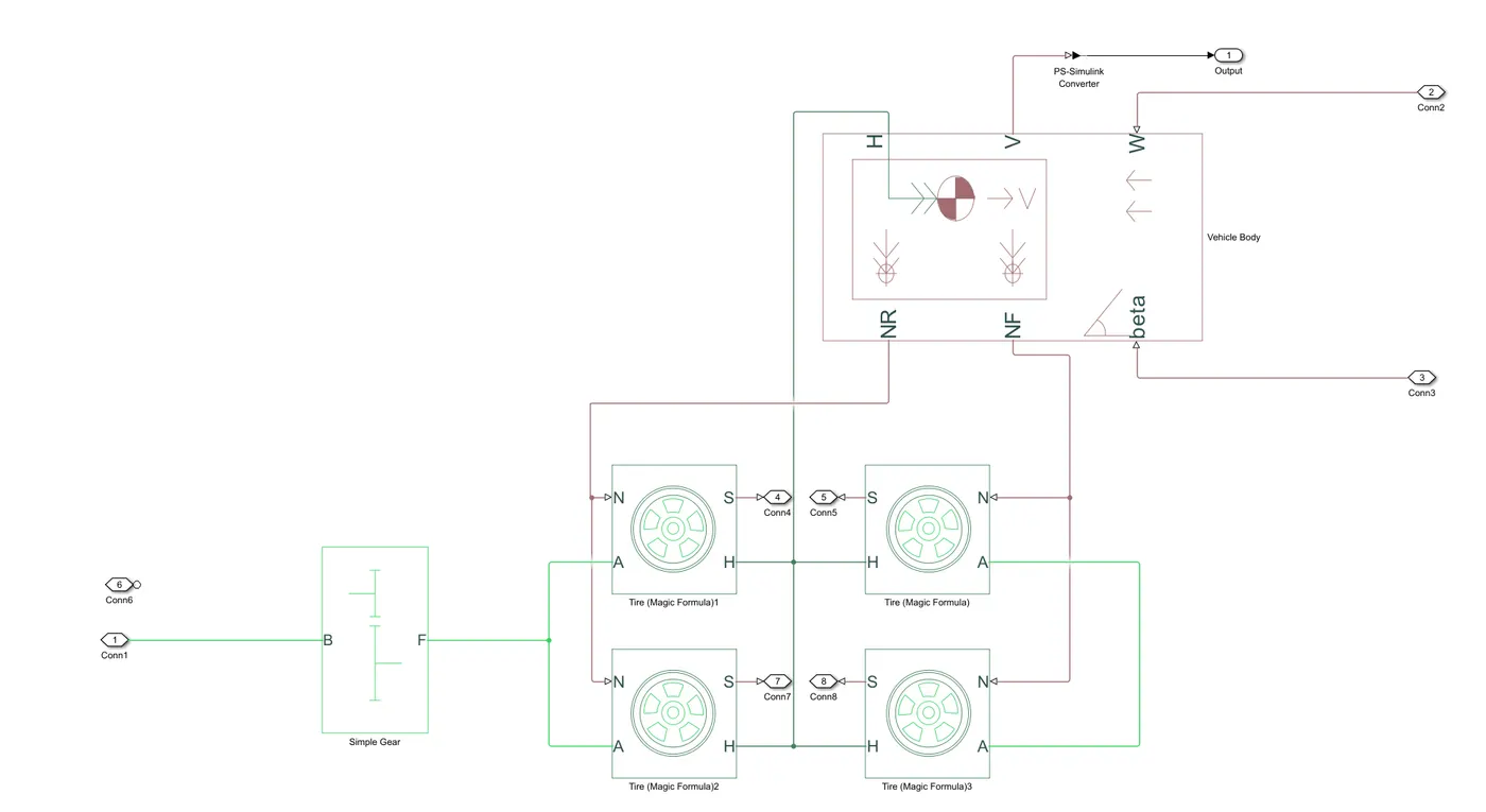
8. Vehicle Body
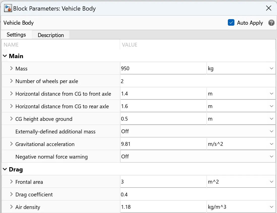
This block represents a two-axle vehicle body in longitudinal motion, accounting for body mass, aerodynamic drag, road incline, and weight distribution between axles due to acceleration and road profile. The vehicle can have a different number of wheels on each axle or the same number. It also offers optional features such as pitch dynamics, suspension dynamics, or additional variable mass and inertia. The vehicle does not move vertically relative to the ground.
Connection H is a mechanical translational conserving port associated with the vehicle body's horizontal motion, where the traction force generated by the tires should be connected. Connections V, NF, and NR are physical signal output ports that provide the vehicle's velocity and the normal forces on the front and rear wheels, respectively, with downward wheel forces considered positive. Connections W and beta serve as physical signal input ports for headwind speed and road inclination angle. If variable mass is modeled, input ports CG and M become available: CG takes a two-element vector indicating the x and y distance offsets from the vehicle's center of gravity (CG) to the additional load's CG, while M represents the additional mass. If both variable mass and pitch dynamics are modeled, the port J accepts the inertia of the additional mass about its CG.
9. Simple Gear
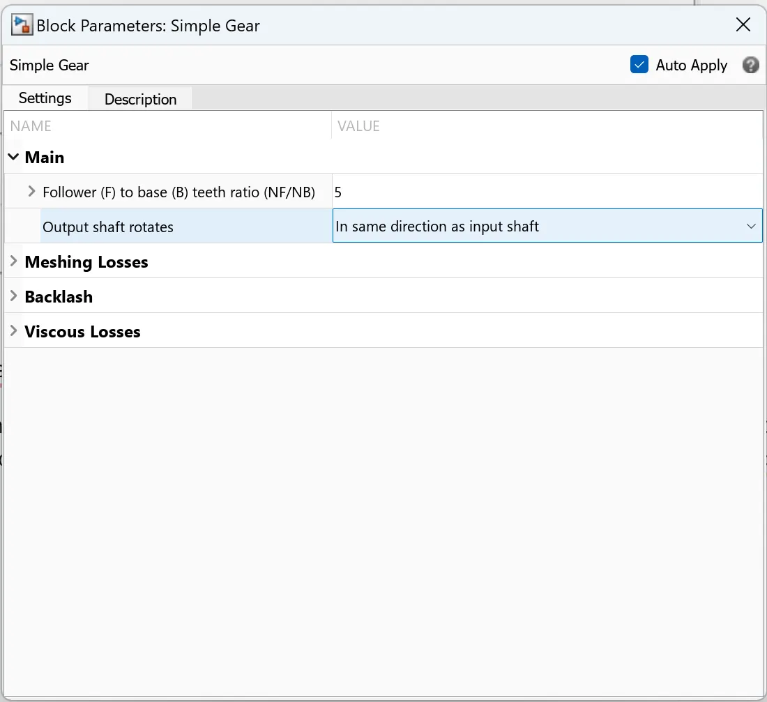
This block represents a fixed-ratio gear or gearbox without modelling inertia or compliance. It optionally allows for the inclusion of gear meshing effects, backlash, and viscous bearing losses.
Connections B (base) and F (follower) are mechanical rotational conserving ports. The relationship between the rotation directions of the base and follower is determined by the Output shaft rotates parameter. Thermal effects can also be included by setting the friction model to a temperature-dependent option, which will expose the thermal conserving port H.
10. Tire (magic formula)
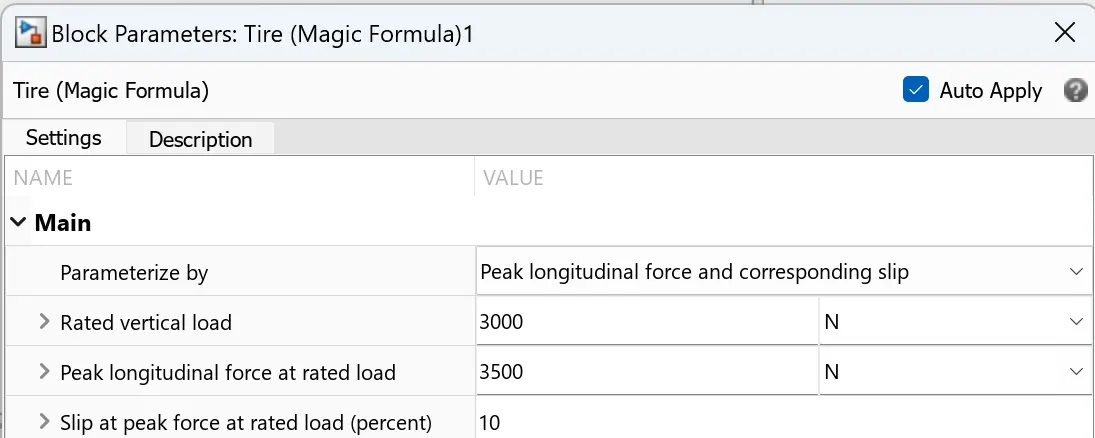
This block represents the longitudinal behavior of a highway tire characterized by the tire Magic Formula. It can optionally account for tire inertia, compliance, and rolling resistance. The scaling effects can also be included when the Parameterize by setting is Load-dependent Magic Formula coefficients or when the Effective rolling radius model is set to Load and velocity-dependent Magic Formula.
Connection A is the mechanical rotational conserving port for the wheel axle, while Connection H is the mechanical translational conserving port for the wheel hub, through which the tire's thrust is applied to the vehicle. Connection N is a physical signal input port that applies the normal force acting on the tire, with positive values indicating downward force. Connection S is a physical signal output port that provides information on tire slip. The physical signal port M can be exposed by setting Parameterize by to Physical signal Magic Formula coefficients, allowing it to accept a four-element vector corresponding to the B, C, D, and E coefficients of the Magic Formula.
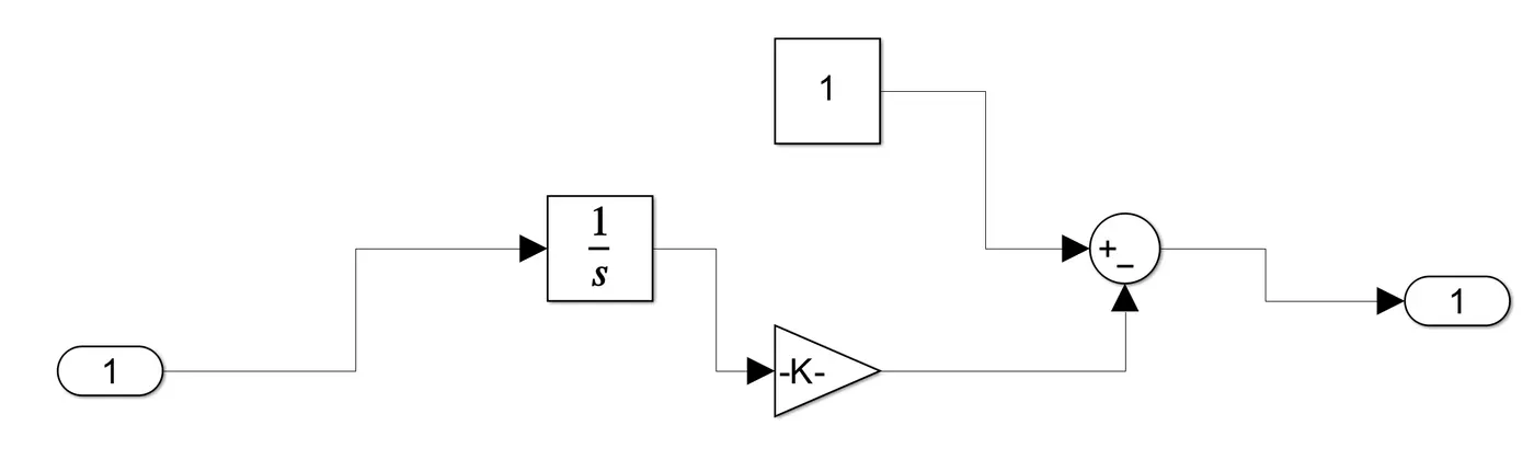
State of Charge Configuration
Vehicle Body Configuration
Results:
The simulation running time was set for 2474 s which is equal to the input drive cycle. Scopes were used to analyze different outputs such as the SOC of the battery, the speed of the vehicle and the reference velocity from the Multiport switch and the distance covered by the vehicle during the simulation.
1. Plot of Reference Speed (from multiport switch) and the speed of the vehicle vs Time:
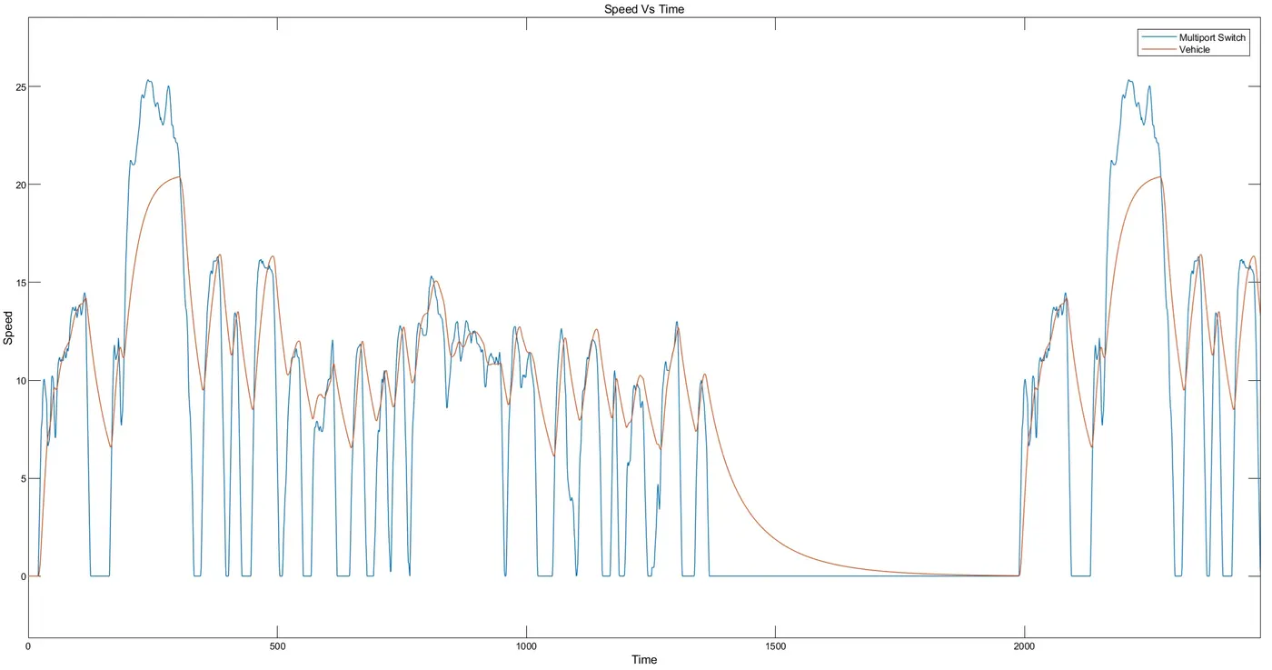
It can be seen that the vehicle's speed closely matches the peak velocities defined by the drive cycle, except around 250 seconds and 2100 seconds. However, it struggles to match the minimum velocities in the drive cycle. The longitudinal speed tracking controller generates normalized acceleration and braking commands based on the reference and feedback velocities. Although the drive cycle includes frequent braking and acceleration, the vehicle's inertia causes a delay in deceleration and subsequent acceleration. Adjusting the parameters of the Longitudinal Driver through multiple iterations can help fine-tune the vehicle speed to better match the reference speed.
2. Plot of Distance vs Time
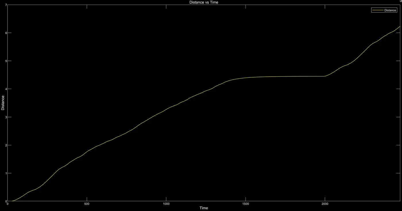
A total distance of 6.23 Km is travelled during the simulation.
Battery State of the Charge
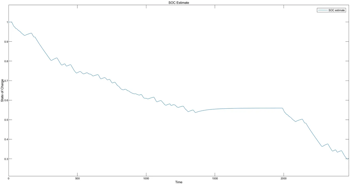
If the total State of Charge (SOC) is considered to be 1, it can be seen that by the end of the simulation, it drops to 0.3, indicating that 70% of the battery has been used, but it has not been fully depleted, allowing the vehicle to continue operating. Additionally, the battery SOC increased during deceleration due to the enabled regenerative braking.
Conclusion:
An electric vehicle model was created, and simulations were performed using the standard FTP75 drive cycle. Throughout the simulation, the battery state of charge (SOC), distance traveled, and actual vehicle speed were tracked and analyzed. The key takeaways from this simulation include:
Developing an electric vehicle model and performing 1D simulations using MATLAB/Simulink.
Gaining insights into how various components and parameters affect vehicle dynamics, including SOC, distance, and speed.
References:
[1] Yong, J. Y., Ramachandaramurthy, V. K., Tan, K. M., & Mithulananthan, N. (2015). A review on the state-of-the-art technologies of electric vehicle, its impacts and prospects. Renewable and sustainable energy reviews, 49, 365-385.