Final Project: Design of an Electric Vehicle
| Final Project: Design of an Electric Vehicle |
AIM : To create a MATLAB model of electric car which uses a Battery and a DC Motor.
THEORY :
Block Diagram of an EV :-
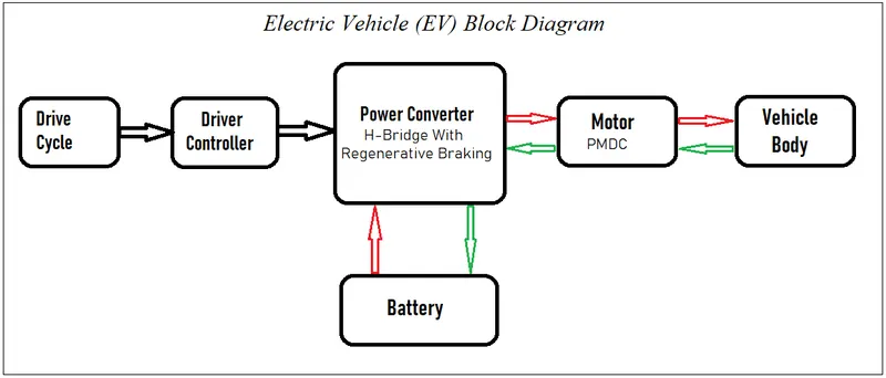
Taking a look at each block -
1 - Vehicle Body.
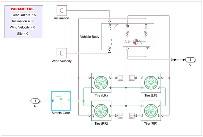
- R is Rotational input port from motor, V is Vehicle Velocity output port.
- It is modeled using 4 tires block and and one vehicle body block. [Rear Wheel Drive]
- Vehicle Body Block - It has 2 physical system (PS) input ports headwind Speed (W), Inclination (beta).
3 PS output ports Vehicle Velocity (V), Normal Force Front (NF), Normal Force Rear (NR).
It represents 2 axle vehicle body in logitudinal motion (i.e. vertical motion is absent).
H port - mechanical translational conserving port represents horizontal motion.
It is connected to all the tires representing 2 axle.
W port - modelled using PS Constant block with 0 value.
beta port - modelled using PS Constant block with 0 value.
NF port - connected to 2 front tires. NR port - connected to 2 rear tires.
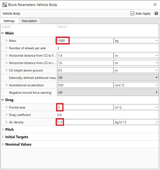
It can be parametered using body mass, aerodynamic drag, road inclination.
|
For this model :- Mass = 1000 kg. Frontal area = 3 `m^2` Air density = 1.3 `(kg)(/m^3)` All other parameters are kept default. |
 |
- Tire Block - It has 3 input ports H : mechanical translational conserving port for wheel hub, through which thrust developed by tire is applied to vehicle.
A : mechanical rotational conserving port for the wheel axle.
connected with Follower gear of Simple Gear block.
N : physical signal port that applies normal force acting on tire.
S : PS output port - reports tire slip. They are terminated here with PS Terminator block as they are not considered in this model.
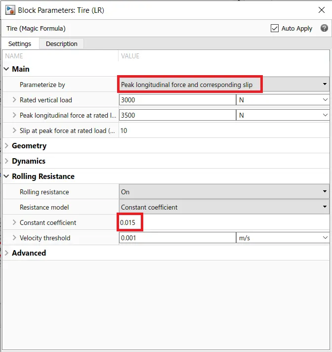
It is built from Tire-Road Interaction (Magic Formula).
|
For this model :- Peak Longitudinal force parameter is used. Rolling Resistance = 0.015 All other parameters are kept default. |
 |
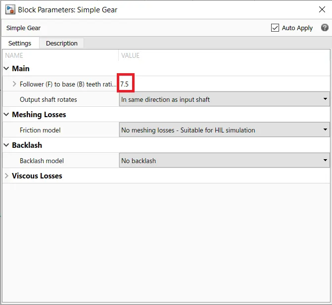
- Simple Gear Block - Port (B) Base & (F) Follower are mechanical rotational conserving port.
B is connected to Motor output, F is connected to Wheel Axle at A port of tire.
They specify the relation between B & F rotation direction with the Output shaft rotates parameter.
It represents a fixed-gear ratio.
|
For this model :- Gear ratio = 7.5 All other parameters are kept default. |
 |
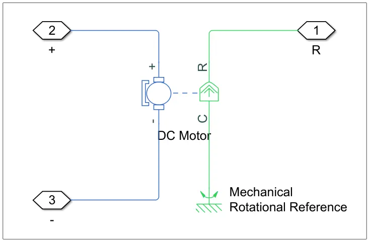
2 - Motor.
|
 |
|
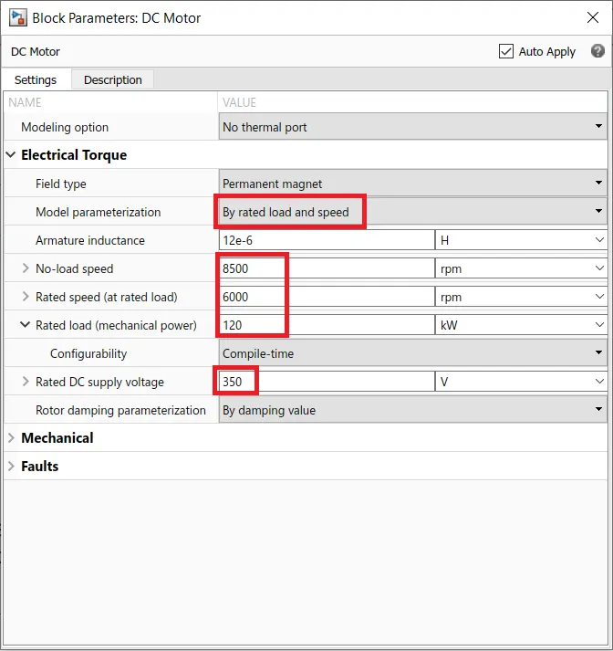
For this model :- Motor block is parametirised by rated load and speed. No load Speed = 8500 rpm Rated Speed = 6000 rpm Rated Load = 120 kW Rated DC Supply = 350 V. All other parameters are kept default. |
 |
3 - Battery.
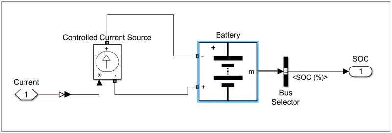
- 1 is input port from Power Converter, 1 output port for SOC.
- It is modelled using a Battery block, Controlled Current Source block, Bus Selector.
- PS-Simulink Block - It converts the input physical signal to a Simulink output signal.
Since the converter circuit is modelled using blocks from different library, it is used to connect to simulink library.
- Controlled Current Source Block - It maintains the specified current through it regardless of voltage across it.
The battery is drained as per the requirement from the DC motor, which is input to this block.
- Bus Selector - It accepts a bus as input and gives multiple output signals.
|
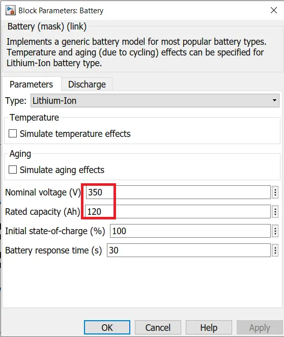
Battery for this model :- Nomial Voltage = 350 V. Rated Capacity = 120 Ah. All other parametes are kept default. |
 |
4 - Power Converter.
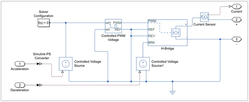
- 2 Input ports : (1) Acceleration & (2) Deceleration from Longitudinal Driver block.
- 3 output ports : (1) Current signal to Battery block. (2) & (3) positive and negative terminal input for DC motor.
- Power converter is modelled using a Controlled PWM Voltage Block, H-Bridge Block, Current Sensor Block, Controlled Voltage Source Block, Solver Configuration Block, Electrical Reference Block. (From Simscape Library)
- Controlled PWM Voltage - It creates a PWM voltage across PWM and Ref ports .
Output voltage is zero when the pulse is low, and is equal to Output voltgae when pulse is high. Duty cycle is set by the input value.
Its input is taken from Controlled Voltage source at ref+ and ref- ports, and output is given to H-bridge from PWM and REF ports.
|
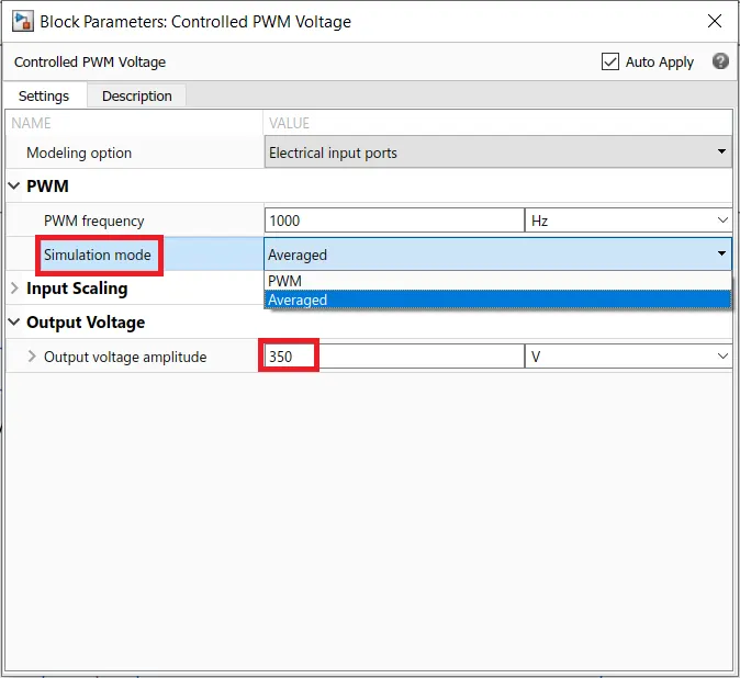
For this model :- Simulation mode = Averaged. (considering simulation time constraint) Output Voltage Amplitude = 350 V |
 |
- H-Bridge Block - It represents a motor drive driven by the Controlled PWM voltage block. Hence both block should be in same simulation mode. (either PWM or Averaged).
In Averaged mode, the PWM port voltage divided by the PWM signal amplitude parameter defines the ratio of the on-time to the PWM period. Using this ratio and assumptions about the load, the block applies an average voltage to the load that achieves the correct average load current.
It has 4 input ports - PWM port : takes PWM voltage input from PWM block.
REF port : It is a reference port.
REV port : It reverses output voltage polarity when its input is greater than Reverse Threshold voltage.
BRK port : It conducts the Freewheeling Diode when its input is greater than the Braking Threshold voltage. Thus enabling regeneration.
It has 2 output ports - (+) & (-) polarity for motor.
|
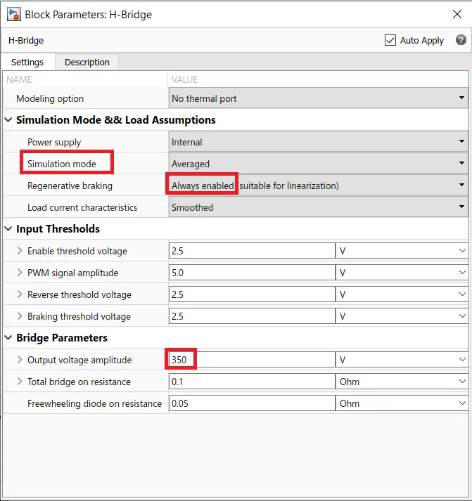
For this model :- Simulation mode = Averaged. Regenerative Braking = Enabled. Output Voltage = 350 V. All other parameters are kept default. |
 |
- Current Sensor Block - It converts current measured in electrical branch into physical signal propotional to the current.
Ports (+) & (-) : conserving electrical ports. Port I : PS port that outputs current.
- Controlled Voltage Source - It maintains the specified voltage at its output regardless of current passing through it.
It has one input port - that takes PS value.
- Simulink-PS Converter - It helps connect Simulink library block to PS block.
In this model Acceleration & Deceleration are inputs from Longitudinal Driver (Simulink Library) connected to PS Controlled voltage source.
- Solver Configuration Block - It specifies the solver parameters for model simulation. Each physical network requires solver settings information for simulation.
- Electrical Reference Block - It represents electrical ground.
5 - Longitudinal Driver.
-
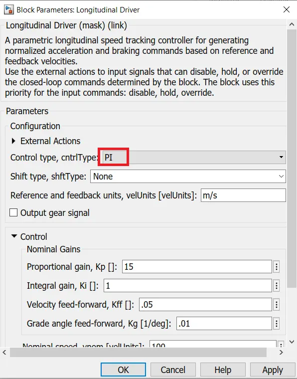
It is a speed tracking controller for generating normalized acceleration and braking commands based on reference and feedback velocities.
- It has 3 inputs : Velocity Reference which takes input reference velocity. In this model it is taken from Drive Cycle.
Velocity Feedback which takes input from feedback to be compared with reference velocity.
Grade which gradeability input.
- It has 3 outputs : Acceleration command, Deceleration Command and Info.
Acceleration command is given as input to Power Converter Block, which controls the voltage applied to the motor.
Deceleration command is also given as input to Power Converter Block, which enables the power converter to regenerate / or feed power back to battery.
Info is terminated in this model, as it is not needed.
|
For this model :- Control type = PI (Proportional & Integral Gain) Values of Kp and Ki are kept default. Grade = 0. |
 |
6 - Drive Cycle.
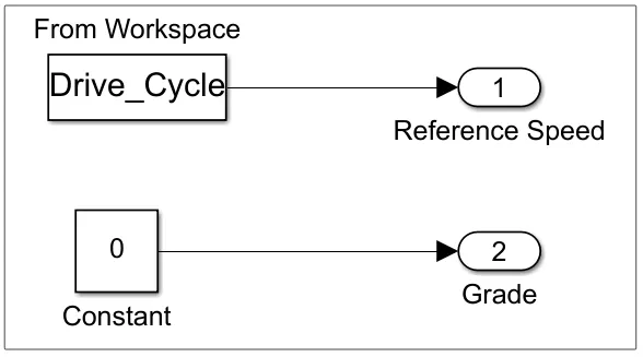 |
- It has 2 outputs : Reference Speed & Grade, given as input to Longitudinal Driver.
- It is modelled using a Constant block and From Workspace block.
- Constant Block - It specifies the constant value of gradeability to longitudinal driver.
- From Workspace Block - It is used to read data [T,V] from workspace, to create a drive cycle.
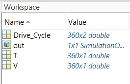
Data is read into workspace from an excel sheet using following MATLAB code.
% Reading Data From Excel Sheet.
T = xlsread ('My Drive cycle (mps).xlsx','A:A');        % Reading A column.
V = xlsread ('My Drive cycle (mps).xlsx','B:B');        % Reading B cloumn.
Drive_Cycle = [T,V]; % Creating Drive Cycle Vector. |
 |
SIMULINK MODEL :-
- All above blocks have been connected respectively to build this model.
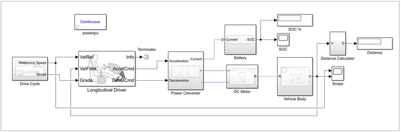
- Display Block - It is used to display the numerical values of SOC as well as Distance travelled.
- Scope Block - It is used to display the graph of Drive Cycle vis-a-vis Vehicle output and SOC.
- Powergui Block - It sets the simulation type, simulation parameters and preferences. Continuous simulation type is used.
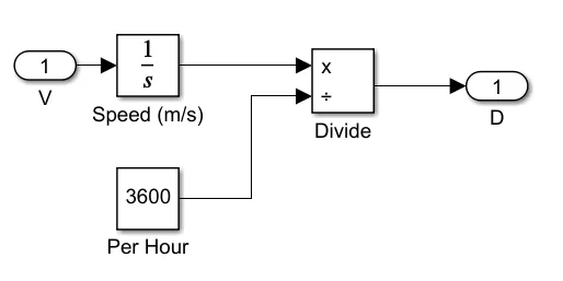
- Distance Calculator Block -
|
It is used to display the distance travelled by the vehicle for a given drive cycle. It is modelled using a Integrator block, constant block, Divide block. Output speed / velocity (m/s) is integrated to get the Distance and is divided by 3600 seconds to get distance in Kilometers. |
 |
OBSERVATION :
- The simulation was run for 360 seconds, as the drive cycle was of 360 seconds.
| Distance Travelled | SOC (%) |
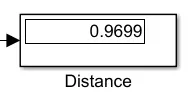 It is almost 1 Km. It is almost 1 Km. |
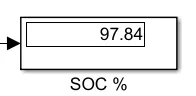 For 1 Km almost 3% soc is used. For 1 Km almost 3% soc is used. |
- Drive Cycle Graph.
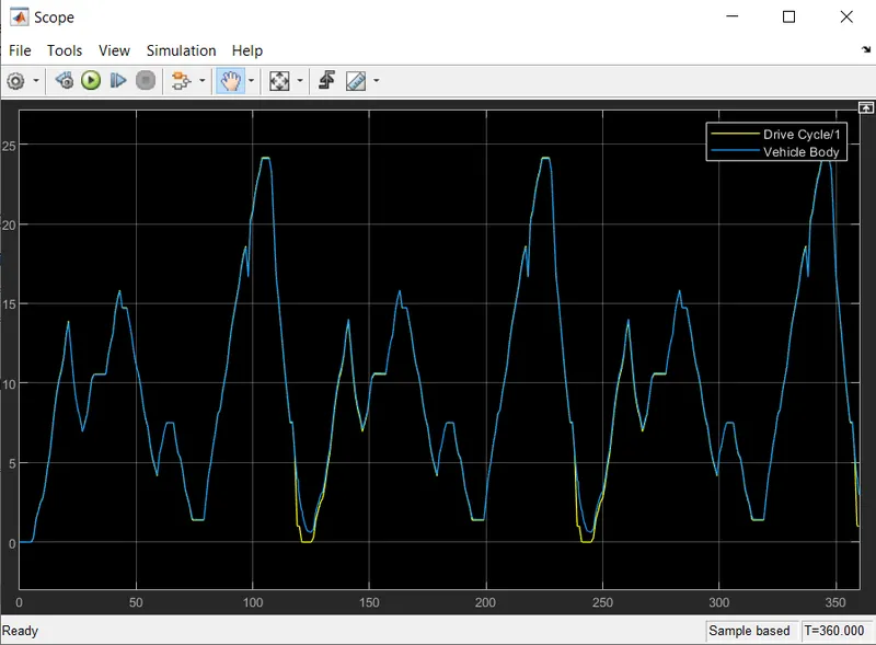
- Above graph shows the output of the simulation of EV Model.
- Yellow line shows the original Drive Cycle and Blue line shows the Vehicle cycle.
- As both the lines are overlapping, it is evident that the vehicle follows the desired path of the Drive Cycle input.
- SOC Graph.
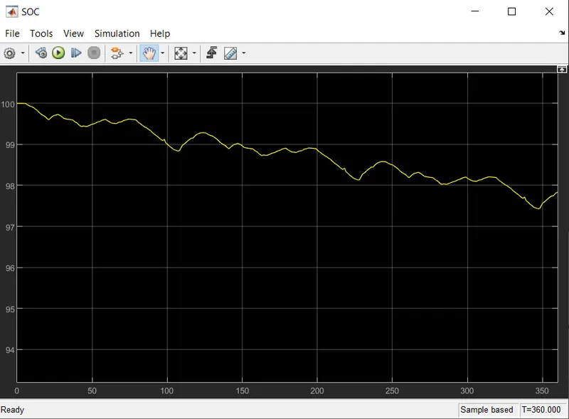
- The battery discharges upto 3 % for 1 Km of distance.
- From the graph it is evident that the battery discharges when current is demanded by the motor, and it recharges when current is fed to it due to regenerative braking.
- Battery SOC reduces when it is discharged while it increases when it is being charged.
CONCLUSION :
As the vehicle is following desired path and desired response to the Drive cycle while discharging the battery when accelerated and charging the battery when brakes are applied to it, it can be concluded that the model is successful.